Moment Conditions and the Generalized Method of Moments
Lecture 11
0.1 Where we are
Where this lecture sits
You have been reading estimators as moment conditions all semester, even if quietly. Lecture 4 noted that the OLS normal equations \(\bX'\be=\bzero\) are a sample moment condition; Lecture 9 wrote IV and 2SLS as \(\E[\mathbf{z}\varepsilon]=\bzero\), one moment per instrument. What was missing was the name and the general machinery. GMM supplies both: it takes the idea you already use — an estimator is whatever makes a set of moment conditions hold in the sample — and turns it into a method, including the two cases the earlier lectures could only gesture at: what to do when there are more moment conditions than parameters, and how to combine them efficiently.
So this is a consolidation, not a new trick. Seen through it, OLS, IV and 2SLS are not three methods but one, with three choices of what to call a moment and how to weight them. The payoff is concrete. Unification: we will derive — not assert — that 2SLS is GMM with a particular weight matrix. Efficiency: Lecture 10 left two debts, and GMM settles both — how to use the moments efficiently when errors are heteroskedastic (where 2SLS is no longer best), and the robust form of the Sargan test, the \(J\)-statistic. A bridge: the same “solve a moment condition” idea reaches forward to maximum likelihood next lecture. Depth stays deliberately light — the goal is the language, not a GMM course.
Not “\(y=\mathbf{x}'\bbeta+\varepsilon\) with assumptions.” The primitive is a set of valid moment conditions \(\E[\mathbf{g}(\mathbf{d}_i,\btheta_0)]=\bzero\), holding only at the true \(\btheta_0\). The parameter is whatever zeroes the population moments; everything else is how we estimate it from the sample.
1 Part I · From moment conditions to an estimator
1.1 The objects
A moment condition: \(\mathbf{d}_i\), \(\mathbf{g}\), and \(\btheta\)
Three objects. The data \(\mathbf{d}_i\) — everything observed for unit \(i\) (here \(\mathbf{d}_i=(y_i,\mathbf{x}_i,\mathbf{z}_i)\)). The parameter \(\btheta\) — the \(k\times1\) vector we want. The moment function \(\mathbf{g}(\mathbf{d}_i,\btheta)\) — an \(\ell\times1\) vector built so that its population mean is zero only at the truth, and estimated by its sample average: \[\underbrace{\E[\mathbf{g}(\mathbf{d}_i,\btheta_0)]=\bzero}_{\ell\text{ population moment conditions}} \qquad\xrightarrow{\ \text{analogy principle}\ }\qquad \underbrace{\bar{\mathbf{g}}_n(\btheta)=\frac1n\sum_{i=1}^n\mathbf{g}(\mathbf{d}_i,\btheta)\ \approx\ \bzero}_{\text{sample analogue}} .\]
Make it concrete with the oldest estimator of all — the mean. Here \(\mathbf{d}_i=y_i\) (a scalar), \(\btheta=\mu\), and \(\mathbf{g}(\mathbf{d}_i,\mu)=y_i-\mu\), so \(\ell=k=1\). The moment condition \(\E[y_i-\mu]=0\) says exactly “\(\mu\) is the population mean”, and it holds at a single value, \(\mu_0=\E[y_i]\). The analogy principle replaces the expectation by the average, \(\frac1n\sum_i(y_i-\mu)=0\), whose solution is the sample mean \(\hat\mu=\bar y\). Nothing more is going on in GMM than this — the only things that change across the examples on the next slide are the choice of \(\mathbf{g}\) and, once \(\ell>k\), how we weight its entries. One note on symbols, to head off a classic confusion: \(\mathbf{d}_i\) (with the subscript \(i\)) is the data for one observation; the bold \(\bW\) that enters later is the weight matrix. They are different things.
1.2 One recipe, many estimators
The same machine, four choices of \(\mathbf{g}\)
| estimator | parameter \(\btheta\) | moment \(\mathbf{g}(\mathbf{d}_i,\btheta)\) | count | weight \(\bW\) |
|---|---|---|---|---|
| mean | \(\mu\) | \(y_i-\mu\) | \(\ell=k=1\) | — |
| OLS | \(\bbeta\) | \(\mathbf{x}_i(y_i-\mathbf{x}_i'\bbeta)\) | \(\ell=k\) | — |
| IV (exact) | \(\bbeta\) | \(\mathbf{z}_i(y_i-\mathbf{x}_i'\bbeta),\ \dim\mathbf{z}_i=k\) | \(\ell=k\) | — |
| 2SLS | \(\bbeta\) | \(\mathbf{z}_i(y_i-\mathbf{x}_i'\bbeta),\ \dim\mathbf{z}_i=\ell>k\) | \(\ell>k\) | \((\bZ'\bZ)^{-1}\) |
Read the table as one machine with a dial. The moment function encodes what you assume is uncorrelated with the error: OLS asserts \(\E[\mathbf{x}\varepsilon]=0\) and so uses \(\mathbf{x}\) as its own instrument; IV asserts \(\E[\mathbf{z}\varepsilon]=0\) and swaps \(\mathbf{z}\) in for the endogenous columns; 2SLS keeps that same \(\mathbf{g}\) but with more instruments than parameters. The counts \(k\) and \(\ell\) are then read off directly, and the weight matrix \(\bW\) enters only for 2SLS — the one over-identified row (\(\ell>k\)). The first three rows are exactly identified (\(\ell=k\)): the moment system is square, so it is solved exactly, \(J\) hits its floor of \(0\), and the weight cancels. Everything in Parts II–IV is about the over-identified case: how to combine surplus moments, how to weight them best, and how to test them.
1.3 The moment system
The equations the moments generate
One equation per instrument — stack them and the matrix form appears: \[\frac1n\sum_{i=1}^n z_{ij}\,(y_i-\mathbf{x}_i'\bbeta)=0,\quad j=1,\dots,\ell \qquad\Longleftrightarrow\qquad \frac1n\,\bZ'(\bY-\bX\bbeta)=\bzero \qquad(\ell\text{ equations},\ k\text{ unknowns}).\] Identification asks whether this system pins \(\bbeta\) down. In population it rearranges to a linear system, \[\E[\mathbf{z}\mathbf{x}']\,\bbeta=\E[\mathbf{z}y],\qquad\text{unique solution}\quad \bbeta_0=(\E[\mathbf{z}\mathbf{x}'])^{-1}\E[\mathbf{z}y]\ \ \textbf{iff}\ \ \rank\E[\mathbf{z}\mathbf{x}']=k .\]
Each instrument contributes one estimating equation, \(\tfrac1n\sum_i z_{ij}(y_i-\mathbf{x}_i'\bbeta)=0\); stacking the \(\ell\) of them is exactly \(\tfrac1n\bZ'(\bY-\bX\bbeta)=\bzero\). So “a moment condition” is not abstract — it is a concrete system of \(\ell\) equations in the \(k\) unknowns \(\bbeta\). Identification is the question of whether that system has a unique solution. Taking expectations and rearranging turns the population version into the linear system \(\E[\mathbf{z}\mathbf{x}']\bbeta=\E[\mathbf{z}y]\), which has the unique solution \(\bbeta_0=(\E[\mathbf{z}\mathbf{x}'])^{-1}\E[\mathbf{z}y]\) precisely when \(\E[\mathbf{z}\mathbf{x}']\) has full rank \(k\) — the same rank condition from Lecture 9, now visible as “the moment system is solvable and the solution is unique.” When rank fails, some combination of \(\bbeta\) leaves every moment unchanged: a flat direction the data cannot resolve. When \(\ell=k\) the system is square and this solution is IV; when \(\ell>k\) the target is still \(k\) unknowns but there are now \(\ell>k\) equations — the next slide.
1.4 Exactly vs. over-identified
When \(\ell>k\): the instruments disagree
One endogenous regressor (\(k=1\)), two instruments (\(\ell=2\)): each instrument gives its own moment equation \(m_j(\beta)=0\), hence its own just-identified IV estimate \(\hat\beta_j\) — and with \(\ell>k\) they disagree.
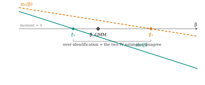
In symbols, each instrument’s moment and its single-instrument IV estimate are \[m_j(\beta)=\frac1n\sum_i z_{ij}(y_i-x_i\beta)=0\ \Rightarrow\ \hat\beta_j=\frac{\sum_i z_{ij}y_i}{\sum_i z_{ij}x_i},\qquad j=1,2.\] This is over-identification stripped to one picture. With \(k=1\) and \(\ell=2\) you have two estimating equations but only one free parameter (\(\beta\)) to satisfy them with. Each equation, read alone, is an exactly-identified IV estimator using a single instrument, and lands at its own number \(\hat\beta_j=\sum_i z_{ij}y_i/\sum_i z_{ij}x_i\). If both instruments were perfect and the sample infinite, the two numbers would coincide at \(\beta_0\); in any real sample they differ, and under \(\ell>k\) there is simply no value of that one parameter that sets both sample moments to zero. The naive responses — keep one instrument, or average the two by hand — either throw away information or pick an arbitrary split. GMM makes the split principled: it minimizes a weighted size of the whole moment vector \(\bar{\mathbf{g}}_n(\beta)=(m_1(\beta),m_2(\beta))'\), landing \(\hat\beta_{\text{GMM}}\) between \(\hat\beta_1\) and \(\hat\beta_2\), tilted toward the moment we trust more. “Trust” is exactly what \(\bW\) encodes — and Part III shows the optimal tilt is by the inverse variance of the moments. The disagreement is not a nuisance to hide: its size is the basis of the overidentification (\(J\)) test in Part IV.
1.5 The GMM criterion
Minimize a weighted distance of the moments
\[\boxed{\ J(\btheta)=n\,\bar{\mathbf{g}}_n(\btheta)'\,\bW\,\bar{\mathbf{g}}_n(\btheta)\ },\qquad \bW\succ0, \qquad \hat\btheta_{\text{GMM}}=\argmin_{\btheta} J(\btheta).\]
\(J\) has no closed form in general ⇒ numerical minimization (gancho: a otimização da Aula 13). The linear case (OLS/IV/2SLS) is the exception — \(\bar{\mathbf{g}}_n\) is linear in \(\btheta\), so \(\hat\btheta\) has a closed form (Part II).
The criterion \(J(\btheta)\) is just the squared length of the moment vector, measured in the metric \(\bW\): when the moments are near zero \(J\) is small, and minimizing it drives all \(\ell\) moments toward zero at once. \(\bW\) fixes the exchange rate between moments that conflict — how much a miss on one is worth against a miss on another, and how their correlations count. Two features organize everything that follows. In the just-identified case the vector can be driven exactly to zero, so \(J\) reaches its floor of \(0\) and the weight never matters — we recover method of moments and IV. In the over-identified case \(J>0\) at the optimum and the choice of \(\bW\) changes the answer: Part III finds the \(\bW\) that makes the estimator most precise, and Part IV shows that the leftover minimized value \(J(\hat\btheta)\) is itself the overidentification test.
2 Part II · OLS, IV and 2SLS are all GMM
2.1 Least squares
OLS is just-identified GMM
Take \(\mathbf{g}(\mathbf{d}_i,\bbeta)=\mathbf{x}_i(y_i-\mathbf{x}_i'\bbeta)\), so \(\ell=k\). The sample moment is the OLS normal equation: \[\bar{\mathbf{g}}_n(\bbeta)=\tfrac1n\bX'(\bY-\bX\bbeta)=\bzero \ \Longleftrightarrow\ \bX'\be=\bzero \ \Longrightarrow\ \hat\btheta_{\text{GMM}}=\bb_{\text{OLS}} .\]
Lecture 4 split OLS into two routes — minimize the sum of squares, or solve the moment \(\bX'\be=\bzero\). GMM is the second route made general: every estimator in this course is “solve (or get as close as possible to) a moment condition.”
2.2 Instrumental variables
IV is just-identified GMM
Swap the instrument: \(\mathbf{g}=\mathbf{z}_i(y_i-\mathbf{x}_i'\bbeta)\) with \(\ell=k\). Then \[\bar{\mathbf{g}}_n(\bbeta)=\tfrac1n\bZ'(\bY-\bX\bbeta)=\bzero \ \Longrightarrow\ \hat\btheta_{\text{GMM}}=\bb_{\text{IV}}=(\bZ'\bX)^{-1}\bZ'\bY .\]
2.3 Two-stage least squares
2SLS is over-identified GMM with a specific weight
Now \(\ell>k\) with \(\mathbf{g}=\mathbf{z}_i(y_i-\mathbf{x}_i'\bbeta)\). Minimizing \(J\) with \(\bW=(\bZ'\bZ/n)^{-1}\) gives the closed form \[\hat\btheta_{\text{GMM}}(\bW)=\big(\bX'\bZ\,\bW\,\bZ'\bX\big)^{-1}\bX'\bZ\,\bW\,\bZ'\bY \ \xrightarrow{\ \bW=(\bZ'\bZ)^{-1}\ }\ \bb_{\text{2SLS}}=\big(\bX'\bP_{\bZ}\bX\big)^{-1}\bX'\bP_{\bZ}\bY .\]
| Estimator | moment \(\mathbf{g}(\mathbf{d}_i,\btheta)\) | count | weight \(\bW\) |
|---|---|---|---|
| OLS | \(\mathbf{x}(y-\mathbf{x}'\bbeta)\) | \(\ell=k\) | irrelevant |
| IV | \(\mathbf{z}(y-\mathbf{x}'\bbeta)\) | \(\ell=k\) | irrelevant |
| 2SLS | \(\mathbf{z}(y-\mathbf{x}'\bbeta)\) | \(\ell>k\) | \((\bZ'\bZ)^{-1}\) |
| Efficient GMM | \(\mathbf{z}(y-\mathbf{x}'\bbeta)\) | \(\ell>k\) | \(\bS^{-1}\) (Part III) |
3 Part III · Efficient GMM and the optimal weight
3.1 Which weight?
Every weight is consistent — not every weight is efficient
For any fixed \(\bW\succ0\), \(\hat\btheta_{\text{GMM}}(\bW)\) is consistent (the moments are valid); \(\bW\) only changes the asymptotic variance. So: which \(\bW\) makes it smallest?
The optimal weight is \(\bW^{\*}=\bS^{-1}\)
With \(\bS=\Asyvar\big(\sqrt n\,\bar{\mathbf{g}}_n\big)=\E[\mathbf{g}\mathbf{g}']\) (the long-run variance of the moments), the efficient GMM weight is \(\bW^{\*}=\bS^{-1}\): \[\bS=\sigma^2\bQ_{zz}\ \text{(homosk.)}\ \Rightarrow\ \bW^{\*}=(\sigma^2\bQ_{zz})^{-1}\Rightarrow \textbf{2SLS efficient};\qquad \bS=\E[\mathbf{z}\mathbf{z}'\varepsilon^2]=\bOmega\ \text{(heterosk.)}\ \Rightarrow\ \textbf{2SLS not efficient.}\]
3.2 Making it feasible
Feasible two-step GMM
\(\bS\) is unknown, so estimate it: \[\text{Step 1: } \bW=(\bZ'\bZ)^{-1}\ \Rightarrow\ \hat\btheta^{(1)}\ \Rightarrow\ \hat\varepsilon_i;\qquad \hat\bS=\tfrac1n\sum_i \mathbf{z}_i\mathbf{z}_i'\hat\varepsilon_i^2;\qquad \text{Step 2: } \bW=\hat\bS^{-1}\ \Rightarrow\ \hat\btheta^{(2)}.\]
3.3 The distribution
Asymptotic normality of GMM
With \(\bG=\E[\partial \mathbf{g}/\partial\btheta']\) (the moment Jacobian — the “bread”): \[\sqrt n\,(\hat\btheta_{\text{GMM}}-\btheta_0)\ \dto\ \Normal\!\Big(\bzero,\ (\bG'\bW\bG)^{-1}\bG'\bW\bS\bW\bG(\bG'\bW\bG)^{-1}\Big) \ \xrightarrow{\ \bW=\bS^{-1}\ }\ \Normal\!\big(\bzero,\ (\bG'\bS^{-1}\bG)^{-1}\big).\]
4 Part IV · Testing the overidentifying restrictions
4.1 The J-test
Overidentification test: the \(J\)-statistic
When \(\ell>k\), the surplus \(\ell-k\) moments are testable. At the efficient GMM estimate, \[J=n\,\bar{\mathbf{g}}_n(\hat\btheta)'\,\hat\bS^{-1}\,\bar{\mathbf{g}}_n(\hat\btheta)\ \dto\ \chi^2_{\ell-k} \quad\text{under } H_0:\ \E[\mathbf{g}(\mathbf{d}_i,\btheta_0)]=\bzero .\]
The Lecture 10 Sargan (\(n R^2\), \(\chi^2_{\ell-k}\)) is exactly this \(J\) under homoskedastic moments. GMM gives its general, robust form — and explains why it is \(\chi^2_{\ell-k}\): \(\ell\) moments minus the \(k\) directions the estimator already forces to zero.
5 Part V · GMM in practice, and the bigger family
5.1 Where GMM is used
Structural vs. design-based: where GMM lives today
GMM did not fade — it split. Its place today depends entirely on which kind of empirical work you do.
The honest status. A student trained in the modern causal toolkit could reasonably think GMM is dated — and, in that corner of the field, the instinct is right. Design-based applied micro has largely abandoned over-identified efficient GMM in favour of just-identified IV reported transparently (“show the first stage, show each instrument’s estimate, do not GMM-combine them”). The reason is not fashion: the efficient two-step estimator weights the moments by an estimated \(\hat\bS^{-1}\), which is noisy in realistic samples and feeds back as bias — the same finite-sample fragility that Lecture 10’s weak- and many-instrument problems are about. Because the credibility revolution prizes robustness and transparency over squeezing out the last drop of efficiency, pooling instruments through a weight matrix is exactly the trade it declines to make.
But GMM never left structural economics. Wherever a model implies moments — a demand system (Berry, Levinsohn & Pakes), a consumption Euler equation (Hansen–Singleton), an asset-pricing stochastic discount factor (Cochrane) — estimation is choosing parameters so that model moments match data moments. When those moments have no closed form, the simulated method of moments (SMM) / indirect inference simulates them. This is a large, active part of the field, and it is GMM through and through.
And as a language it is permanent. The unifying lesson of this lecture — that OLS, IV and 2SLS are one object — is why GMM stays in the course even for students who will only ever run a design-based study: it is the account that makes every linear estimator legible, and, next lecture, the bridge to maximum likelihood.
5.2 Z-estimation
Moment estimators as one family
Estimators that solve \(\tfrac1n\sum_i \boldsymbol{\psi}(\mathbf{d}_i,\btheta)=\bzero\) are Z-estimators (\(Z\) for zero). OLS, IV — and, next lecture, MLE (score \(=\bzero\)) — are all of this family; GMM extends it to the over-identified case (\(\ell>k\)).
The thread continues: minimize a criterion (OLS, GMM) or solve a moment / maximize a likelihood (IV, MLE) — all extremum / M-estimators. Lecture 12 names the family and derives MLE inside it.
6 Summary
What to take away
- A parameter is whatever zeroes the population moments \(\E[\mathbf{g}(W,\btheta_0)]=\bzero\); estimate by the sample analogue.
- With more moments than parameters (\(\ell>k\)) you cannot zero them all — minimize the weighted criterion \(J(\btheta)=n\,\bar{\mathbf{g}}_n'\bW\bar{\mathbf{g}}_n\).
- OLS, IV and 2SLS are GMM with specific \((\mathbf{g},\bW)\) — 2SLS is GMM with \(\bW=(\bZ'\bZ)^{-1}\).
- The optimal weight is \(\bS^{-1}\) (inverse variance of the moments); it matters under heteroskedasticity, where 2SLS is no longer efficient.
- The \(J\)-test (\(\chi^2_{\ell-k}\)) is the robust Sargan: it checks the surplus moments’ mutual consistency — it falsifies, never confirms.
The original theory is Hansen (1982). In structural work GMM/SMM is standard: demand estimation (Berry et al. 1995), consumption Euler equations (Hansen and Singleton 1982), and the asset-pricing SDF framework. In dynamic panels, Arellano–Bond and system GMM (Arellano and Bond 1991) are powerful but prone to instrument proliferation (Roodman 2009). The design-based retreat reflects the finite-sample cost of the estimated optimal weight (Altonji and Segal 1996) — the Lecture 10 theme, once more.