Finite-Sample Properties and the Gauss-Markov Theorem
Lecture 4
1 Where we are
Where this lecture sits
DGPIdentificationEstimationAsymptoticsInference
Computation
Lecture 3 built \(\bb = (\bX'\bX)^{-1}\bX'\bY\) out of pure algebra: it exists for any design of full column rank, whether or not the model is true. We now ask what it is good for.
That question is statistical, so the DGP comes back. Everything below is a statement about the distribution \(\bb\) inherits from the sampling process — never about the number you computed from the one sample in front of you. Lecture 3 lived entirely in the algebra; this lecture is the first in which probability re-enters.
2 The sampling distribution
The estimator is a random variable
The estimate you compute is one number. The estimator is a function of the sample, and the sample is random — so a different draw gives a different \(\bb\).
Imagine drawing many independent samples from the same DGP and recomputing \(\bb\) in each. The spread of values you would get is the sampling distribution of \(\bb\). Every claim this lecture makes — unbiased, efficient, precise — is a statement about that distribution, not about the one number in front of you. This is the central abstraction of estimation theory, and the reason the DGP, absent from Lecture 3, is back.
Which moments do we need?
We cannot write the whole sampling distribution from A1–A4 alone — that needs the normality assumption A6, which we add at the end of this lecture. But we can already compute its moments, and the first two answer the questions that matter.
A distribution is summarised, in increasing detail, by its moments. The first — the mean — tells us whether the estimator is centred on the parameter it targets; any gap is bias. The second — the variance — tells us how far a typical estimate falls from that centre, and is what standard errors report. The two combine into mean squared error, \(\text{MSE}(\bb) = \text{bias}^2 + \Var[\bb]\), the standard scalar verdict on an estimator. Higher moments and the full shape would let us test hypotheses, but they demand normal disturbances or a large sample. So the plan is simple: compute the first moment, then the second, and see how far that gets us.
3 The first moment: the mean
What we are entitled to assume
What is the DGP?
\(y_i = \mathbf{x}_i'\bbeta + \varepsilon_i\) with \((y_i, \mathbf{x}_i)\) i.i.d., \(\rank(\bX) = K\) (A2) and \(\E[\beps \mid \bX] = \bzero\) (A3).
Nothing is assumed about \(\Var[\beps \mid \bX]\).
That silence is deliberate, and it is where this lecture departs from the traditional treatment.
Most presentations assume \(\Var[\beps \mid \bX] = \sigma^2\bI\) from the outset and relax it much later, as though heteroskedasticity were a defect to be repaired. We follow Hansen: the general case first, the constant-variance case as the special one. The pay-off arrives a few slides from now, when the variance formula turns out to need no such assumption.
The sampling error
Everything in this lecture follows from one substitution. Writing \(\bY = \bX\bbeta + \beps\),
\[\bb = \bbeta + \eqt{a}{(\bX'\bX)^{-1}\bX'}\eqt{b}{\beps}\]
a
A fixed matrix once \(\bX\) is given — it carries no randomness of its own.
b
The disturbance. All of the sampling variability of \(\bb\) enters here, and nowhere else.
The estimator equals the truth plus a term linear in \(\beps\). Unbiasedness, variance and efficiency are all read off that single term.
The first property
Theorem 1 (Unbiasedness of least squares) Under A1–A3, \(\E[\bb \mid \bX] = \bbeta\), and therefore \(\E[\bb] = \bbeta\).
On the Board
Worked on the board. The skeleton:
Proof. Take conditional expectations in the decomposition above. The matrix \((\bX'\bX)^{-1}\bX'\) is fixed given \(\bX\), so it passes outside, leaving \((\bX'\bX)^{-1}\bX'\E[\beps \mid \bX] = \bzero\) by A3. The unconditional statement follows by iterated expectations. \(\square\)
Read the proof again
Notice which assumption did the work: A3 alone. Not homoskedasticity, not normality, not even large samples. Unbiasedness is exactly as strong as the exogeneity assumption behind it — no stronger, and no weaker.
Seeing unbiasedness
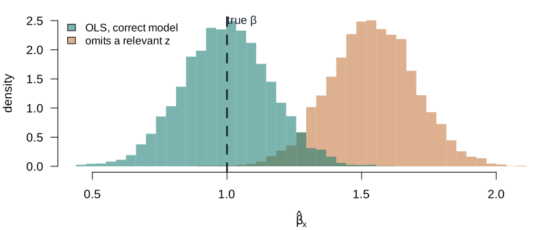
Unbiasedness is a statement about the distribution, not any one estimate. Draw 5,000 samples from a DGP with a known slope \(\beta = 1\) and recompute \(\bb\) in each:
No single run reveals bias: any one estimate can land anywhere under either curve. Only the distribution shows it — the teal mean sits on \(\beta\), the amber mean does not. This is exactly why unbiasedness had to be defined as a property of \(\E[\bb \mid \bX]\), and it is the picture to carry into the omitted-variable algebra that follows: the amber shift is \(\mathbf{p}_{X\cdot z}\gamma\).
4 Omitted variables
When a regressor is left out
Unbiasedness needed only A3. The most common way A3 fails in practice is not exotic: a variable that belongs in the model is left out. Lecture 2 flagged this as the leading example of an exogeneity failure and promised the derivation here.
What is the DGP?
The true model is \(\bY = \bX\bbeta + \mathbf{z}\gamma + \beps\) with \(\E[\beps \mid \bX, \mathbf{z}] = \bzero\), but we regress \(\bY\) on \(\bX\) only, leaving out the relevant \(\mathbf{z}\).
The bias, derived
Substituting the true model into \(\bb = (\bX'\bX)^{-1}\bX'\bY\),
\[\bb = \bbeta + \underbrace{(\bX'\bX)^{-1}\bX'\mathbf{z}}_{\mathbf{p}_{X\cdot z}}\gamma + (\bX'\bX)^{-1}\bX'\beps,\]
so taking expectations conditional on \(\bX\) and \(\mathbf{z}\),
Theorem 2 (Omitted-variable bias) \[\E[\bb \mid \bX, \mathbf{z}] = \bbeta + \mathbf{p}_{X\cdot z}\,\gamma, \qquad \mathbf{p}_{X\cdot z} = (\bX'\bX)^{-1}\bX'\mathbf{z}.\]
The bias is the regression of the omitted variable on the included ones, scaled by the omitted variable’s own coefficient \(\gamma\). It vanishes iff \(\gamma = 0\) (the variable was irrelevant) or \(\bX'\mathbf{z} = \bzero\) (it is orthogonal to every included regressor).
Reading the bias one coefficient at a time
\(\mathbf{p}_{X\cdot z}\) is itself a vector of regression coefficients — exactly the object Frisch–Waugh–Lovell describes. By the single-extra-regressor corollary of Lecture 3, the bias in a single coefficient \(b_k\) is
\[\E[b_k \mid \bX, \mathbf{z}] = \beta_k + \gamma\,\frac{\Cov(\mathbf{z}, x_k \mid \text{other }x)}{\Var(x_k \mid \text{other }x)}.\]
The fraction is the coefficient from regressing the omitted variable on \(x_k\) after partialling out the other regressors — the partialled-out covariance over the partialled-out variance, in the \(z_*, x_{k*}\) notation of Lecture 3. The direction of the bias is therefore the sign of \(\gamma\) times the sign of that partial covariance, and its size grows with both.
The sign of the bias
Example 1 (Ability bias in the returns to education) \[\text{Income} = \beta_0 + \beta_1\,\text{Educ} + \beta_2\,\text{age} + \beta_3\,\text{age}^2 + \beta_4\,\text{Ability} + \varepsilon.\]
Ability is unobserved, so we omit it. Then \[\E[b_1 \mid \bX, \text{Ability}] = \beta_1 + \beta_4\,\frac{\Cov(\text{Ability}, \text{Educ} \mid \text{age}, \text{age}^2)}{\Var(\text{Educ} \mid \text{age}, \text{age}^2)}.\] If more able people earn more (\(\beta_4 > 0\)) and also study more (positive partial covariance), \(b_1\) is biased upward: the return to schooling is overstated because it absorbs the return to ability.
5 The second moment: the variance
The general case, not the convenient one
Unbiasedness says the estimates centre on the truth. It says nothing about how far they scatter — and scatter is what standard errors report.
Theorem 3 (Variance of least squares) Let \(\bD = \E[\beps\beps' \mid \bX]\) be the \(n\times n\) conditional variance matrix of the disturbances, with no restriction on its form. Then \[\Var[\bb \mid \bX] = (\bX'\bX)^{-1}\,\bX'\bD\bX\,(\bX'\bX)^{-1}.\]
Proof. \(\bb - \bbeta = (\bX'\bX)^{-1}\bX'\beps\) is linear in \(\beps\); apply \(\Var[\bA\beps] = \bA\,\Var[\beps\mid\bX]\,\bA'\) with \(\bA = (\bX'\bX)^{-1}\bX'\) and \(\Var[\beps\mid\bX] = \bD\). \(\square\)
The expression has a bread–filling–bread shape and is universally called the sandwich formula. It holds under A1–A3 alone — the same assumptions as unbiasedness, and no more.
Two matrices, two sizes, and it pays to keep them apart. \(\bD = \E[\beps\beps'\mid\bX]\) is \(n \times n\) — one entry per pair of observations. The filling \(\bX'\bD\bX\) is only \(K \times K\) — the sandwich never needs all of \(\bD\), just how it weights the regressors. It is this \(K \times K\) filling, in its per-observation form \(\bOmega = \E[\varepsilon^2\mathbf{x}\mathbf{x}']\), that Lecture 5 works with directly.
Conditional, and unconditional
Everything here conditions on \(\bX\). Averaging over the design gives the unconditional variance, and the law of total variance is unusually clean, because the first moment is constant: \[\Var[\bb] = \E\big[\Var[\bb \mid \bX]\big] + \underbrace{\Var\big[\E[\bb \mid \bX]\big]}_{=\ \bzero} = \E\big[\Var[\bb \mid \bX]\big].\]
The second term vanishes because least squares is unbiased: \(\E[\bb \mid \bX] = \bbeta\) does not vary with \(\bX\), so it contributes no variance. The unconditional variance is then just the average of the conditional one. We nonetheless report conditional standard errors, because \(\bX\) is what we observe — the relevant uncertainty is over the disturbances, with the design held at its realised value.
Adding a restriction on the variance
The model of Lecture 2 constrained the conditional mean and said nothing about the conditional variance. We now constrain the variance too — and give the restriction the name the rest of the course uses.
Definition 1 (A4 · Conditional homoskedasticity) \[\bD = \E[\beps\beps' \mid \bX] = \sigma^2\bI_n,\] which packs two claims together: homoskedasticity, \(\sigma^2(\mathbf{x}_i) = \sigma^2\) for every \(i\), and no correlation across observations, \(\Cov[\varepsilon_i,\varepsilon_j \mid \bX] = 0\) for \(i \neq j\).
What A4 collapses
Under A4 the filling \(\bX'\bD\bX\) becomes \(\bX'(\sigma^2\bI_n)\bX = \sigma^2\bX'\bX\), one factor cancels on each side, and what is left is the formula every textbook opens with: \[\Var[\bb \mid \bX] = \sigma^2(\bX'\bX)^{-1}.\]
Important
The familiar formula is not the general result. It is what the sandwich collapses to when the conditional variance happens to be constant. Teaching it first, and the sandwich later as a repair, gets the logic backwards.
Estimating the variance
Both forms need an estimate. Under A4 it suffices to estimate the scalar \(\sigma^2\).
Theorem 4 (Unbiased estimation of \(\sigma^2\)) Under A1–A4, \(s^2 = \be'\be/(n-K)\) satisfies \(\E[s^2 \mid \bX] = \sigma^2\).
Proof. \(\be = \bM\beps\), so \(\E[\be'\be \mid \bX] = \E[\beps'\bM\beps \mid \bX] = \sigma^2\tr(\bM) = \sigma^2(n-K)\), using \(\rank(\bM) = n-K\) from the properties of \(\bP\) and \(\bM\) in Lecture 3. \(\square\)
The divisor \(n-K\) is not a convention: it is exactly what makes the expectation come out right, and it is the trace of the residual maker from Lecture 3.
Without homoskedasticity
When \(\bD\) is unrestricted there is no single \(\sigma^2\) to estimate — there are \(n\) conditional variances and only \(n\) observations. The way out is that the sandwich needs only the \(K \times K\) filling \(\bX'\bD\bX\), not \(\bD\) itself.
Definition 2 (Heteroskedasticity-robust covariance estimator) \[\widehat{\Var}[\bb \mid \bX] = (\bX'\bX)^{-1}\left(\sum_{i=1}^n e_i^2\,\mathbf{x}_i\mathbf{x}_i'\right)(\bX'\bX)^{-1}.\] Each observation contributes its own squared residual as an estimate of its own variance.
This is White’s estimator. Its justification is asymptotic and belongs to Lecture 5; what matters here is the shape — the middle is a weighted cross-product of the regressors, with the weights supplied by the residuals themselves. Nothing needs to be assumed about how the variances vary.
What leverage is
The corrections about to appear depend on leverage — the \(i\)-th diagonal of the projection (hat) matrix \(\bP = \bX(\bX'\bX)^{-1}\bX'\) built in Lecture 3.
Definition 3 (Leverage) \[h_{ii} = [\bP]_{ii} = \mathbf{x}_i'(\bX'\bX)^{-1}\mathbf{x}_i \in [0,1], \qquad \sum_{i=1}^n h_{ii} = K.\]
Leverage measures how much observation \(i\) pulls its own fitted value, \(\partial \hat y_i/\partial y_i = h_{ii}\); a high value flags an \(\mathbf{x}_i\) far from the centre of the design.
This identity is what the corrections exploit. Because \(\be = \bM\beps\) with \(\bM = \bI - \bP\), the residual at a high-leverage point is shrunk toward zero, and its square underestimates that point’s variance by exactly the factor \(1-h_{ii}\). HC2 divides by \(1-h_{ii}\) to undo the shrinkage exactly; HC3 divides by its square, over-correcting on purpose — which turns out to help precisely when a few influential points are present.
Which robust estimator?
Under the Hood—HC0, HC1, HC2, HC3
The estimator above is HC0. Because \(\E[e_i^2] < \E[\varepsilon_i^2]\) — residuals are shrunk by fitting — it is biased downward in small samples, and several corrections exist:
| Correction | |
|---|---|
| HC0 | \(e_i^2\) |
| HC1 | \(\dfrac{n}{n-K}\,e_i^2\) |
| HC2 | \(\dfrac{e_i^2}{1-h_{ii}}\) |
| HC3 | \(\dfrac{e_i^2}{(1-h_{ii})^2}\) |
HC2 and HC3 divide \(e_i^2\) by \((1-h_{ii})\) and by its square — the biggest corrections fall on the high-leverage points, whose residuals shrink most. The exponent on \((1-h_{ii})\) runs \(0, 1, 2\) across HC0, HC2, HC3; HC4 (Cribari-Neto, 2004) makes it adaptive. Stata’s robust is HC1 and R’s vcovHC defaults to HC3, so “robust standard errors” without a label is ambiguous.
6 Gauss-Markov
Why prefer least squares at all?
The Four Questions—Before the theorem
- What problem are we solving? Many estimators are unbiased. Unbiasedness alone does not choose among them.
- Why does it matter? Without a second criterion, “use OLS” is a convention rather than a result.
- What is the idea? Restrict attention to a class — linear and unbiased — and ask which member has the smallest variance.
- How do we formalise it? Show that any other member exceeds the variance of least squares by a positive semi-definite matrix.
The theorem
Theorem 5 (Gauss-Markov) Under A1–A4, for any estimator \(\tilde{\bbeta} = \bA\bY\) that is linear in \(\bY\) and unbiased conditional on \(\bX\), \[\Var[\tilde{\bbeta} \mid \bX] - \Var[\bb \mid \bX] \;\succeq\; \bzero,\] that is, the difference is positive semi-definite. Least squares is BLUE — the best linear unbiased estimator.
Proof
On the Board
Derived on the board — the longest derivation of the course so far. The skeleton:
Proof. Write \(\bA = (\bX'\bX)^{-1}\bX' + \bD\). Unbiasedness for all \(\bbeta\) forces \(\bD\bX = \bzero\). Computing the variance under A4, the cross terms vanish precisely because of that restriction, leaving \(\sigma^2(\bX'\bX)^{-1} + \sigma^2\bD\bD'\). The second term is positive semi-definite. \(\square\)
What the theorem does and does not say
The result is narrower than its reputation. Each qualifier is load-bearing:
- Linear — in \(\bY\). Nonlinear estimators are not compared, and some beat OLS.
- Unbiased — biased estimators are excluded, and some have lower mean squared error.
- Under A4 — homoskedasticity is essential here, unlike in Theorem 1.
Warning
Gauss-Markov is the one place in this lecture where A4 genuinely cannot be dropped. Under heteroskedasticity least squares remains unbiased but is no longer efficient — GLS is, and that is Lecture 7.
7 A pattern worth naming
Least squares as the first of a family
Researcher's Toolbox—OLS as an M-estimator
We obtained \(\bb\) by minimising \(S(\mathbf{b}) = (\bY - \bX\mathbf{b})'(\bY - \bX\mathbf{b})\) — an instance of \[\hat\btheta = \argmin_{\btheta} Q_n(\btheta).\] Estimators defined this way are M-estimators. Maximum likelihood, in Lecture 13, is another: same shape, different criterion. Much of what we proved today will be proved once more, in that generality, for the whole family.
And the other route
Connection—The other route: a moment condition
Setting the derivative of \(S(\mathbf{b})\) to zero gives \(\bX'\be = \bzero\) — a moment condition, and exactly the sample analogue of the population \(\E[\mathbf{x}e] = \bzero\) derived in Lecture 2. It pins \(\bb\) down without minimising anything: least squares is equally the estimator that forces the sample orthogonality to hold. Estimators defined by such an estimating equation, \(\tfrac1n\sum_i \boldsymbol{\psi}(W_i,\btheta) = \bzero\), are Z-estimators (the method of moments). OLS is both at once — an M-estimator that minimises a criterion and a Z-estimator that solves a moment condition — because differentiating the criterion is what produces the condition. This is the thread to IV (Lecture 10) and GMM (Lecture 12).
8 The whole distribution
One more assumption buys the entire shape
The mean and the variance are all A1–A4 will give. To pin down the whole sampling distribution — every quantile, not just centre and spread — we must say something about the shape of the disturbances. One assumption does it.
Definition 4 (A6 · Conditional normality) \[\beps \mid \bX \;\sim\; \Normal(\bzero,\ \sigma^2\bI_n).\] The disturbances are jointly normal, homoskedastic, and uncorrelated across observations, given the design. This is A4 plus a full distributional shape — strictly stronger than anything assumed so far.
A6 fixes not just the first two moments of \(\beps\) but its entire law. In return it delivers the exact, finite-sample distribution of the estimator — and, once we turn to testing in Lecture 6, of the statistics inference is built on (\(s^2\) and the \(t\)-ratio) — with no appeal to large samples at all. This is the normal regression model, and it is where classical inference comes from.
The exact finite-sample distribution
Since \(\bb - \bbeta = (\bX'\bX)^{-1}\bX'\beps\) is a linear function of a normal vector, it is normal too — exactly, for every \(n\), not just in the limit.
Theorem 6 (Normal regression) Under A1–A4 and A6, conditional on \(\bX\), \[\bb \;\sim\; \Normal\!\big(\bbeta,\ \sigma^2(\bX'\bX)^{-1}\big).\]
The proof is one line: \(\bb - \bbeta = (\bX'\bX)^{-1}\bX'\beps\) is a fixed matrix times the normal vector \(\beps\), and a linear map of a normal is normal — with mean \(\bzero\) and variance \((\bX'\bX)^{-1}\bX'(\sigma^2\bI)\bX(\bX'\bX)^{-1} = \sigma^2(\bX'\bX)^{-1}\).
9 What we have, and what is missing
The scoreboard
| Property | Needs | Holds under heteroskedasticity? |
|---|---|---|
| Unbiasedness | A1–A3 | yes |
| Sandwich variance | A1–A3 | yes |
| \(\sigma^2(\bX'\bX)^{-1}\) | + A4 | no |
| \(s^2\) unbiased for \(\sigma^2\) | + A4 | no |
| Efficiency (Gauss-Markov) | + A4 | no |
| Exact normality of \(\bb\) | + A6 | no |
Read the last column. Only efficiency and the simplified formulas depend on A4, and the exact normal distribution of \(\bb\) on the stronger A6; the estimator itself and its variance do not. That is the whole case for treating robust inference as the default rather than the exception.
The limits of finite-sample theory
Everything today was exact and conditional on \(\bX\) — but the distribution, unlike the two moments, came at a price: assumption A6. That price is steep, and it is where the finite-sample story runs out.
Normal disturbances are rarely a credible description of real data, so the exact distribution of Theorem 6, however elegant, has no guarantee of accuracy. Worse, almost no estimator outside least squares is even unbiased. Both problems have the same resolution, and it is the subject of Lecture 5: stop demanding exact results, let \(n\) grow, and recover a normal distribution for \(\bb\) with no assumption that the errors are normal.
10 Reading
Sources
| Hansen | Chapter 4 — §4.2–4.5 (mean, variance, Gauss-Markov), §4.8–4.10 (covariance estimation, standard errors) |
| Greene | Chapter 4 — the assumptions, omitted-variable bias, and the Gauss-Markov theorem |
Hansen’s Chapter 4 supplies the ordering used here — the general variance first, homoskedasticity as the special case. Greene’s Chapter 4 is the source for the omitted-variable-bias derivation and the classical statement of Gauss-Markov.