Moment Conditions and the Generalized Method of Moments
Lecture 11
PIMES/UFPE
Where we are
Where this lecture sits
- Already a moment condition: Lecture 4 read OLS as \(\bX'\be=\bzero\); Lecture 9 read IV as \(\E[\mathbf{z}\varepsilon]=\bzero\) — GMM names the idea and generalises it.
- Lecture 10 left two IOUs: under heteroskedasticity neither OLS nor 2SLS is efficient; and the robust Sargan. GMM pays both.
- Plan: moments → a weighted criterion → OLS/IV/2SLS as special cases → the optimal weight → the \(J\)-test.
Not “\(y=\mathbf{x}'\bbeta+\varepsilon\) with assumptions.” The primitive is a set of valid moment conditions \(\E[\mathbf{g}(\mathbf{d}_i,\btheta_0)]=\bzero\), holding only at the true \(\btheta_0\). The parameter is whatever zeroes the population moments; everything else is how we estimate it from the sample.
Part I · From moment conditions to an estimator
The objects
A moment condition: \(\mathbf{d}_i\), \(\mathbf{g}\), and \(\btheta\)
Three objects. The data \(\mathbf{d}_i\) — everything observed for unit \(i\) (here \(\mathbf{d}_i=(y_i,\mathbf{x}_i,\mathbf{z}_i)\)). The parameter \(\btheta\) — the \(k\times1\) vector we want. The moment function \(\mathbf{g}(\mathbf{d}_i,\btheta)\) — an \(\ell\times1\) vector built so that its population mean is zero only at the truth, and estimated by its sample average: \[\underbrace{\E[\mathbf{g}(\mathbf{d}_i,\btheta_0)]=\bzero}_{\ell\text{ population moment conditions}} \qquad\xrightarrow{\ \text{analogy principle}\ }\qquad \underbrace{\bar{\mathbf{g}}_n(\btheta)=\frac1n\sum_{i=1}^n\mathbf{g}(\mathbf{d}_i,\btheta)\ \approx\ \bzero}_{\text{sample analogue}} .\]
- Data \(\mathbf{d}_i\) = all you observe for \(i\); parameter \(\btheta\) (\(k\times1\)); moment \(\mathbf{g}\) (\(\ell\times1\)), mean-zero only at \(\btheta_0\).
- Analogy principle: swap \(\E[\cdot]\) for \(\tfrac1n\sum_i\), then solve (if \(\ell=k\)) or compromise (if \(\ell>k\)).
- Heads-up on symbols: \(\mathbf{d}_i\) (subscript \(i\)) is the data; the bold \(\bW\) that appears later is the weight matrix — unrelated objects.
One recipe, many estimators
The same machine, four choices of \(\mathbf{g}\)
| estimator | parameter \(\btheta\) | moment \(\mathbf{g}(\mathbf{d}_i,\btheta)\) | count | weight \(\bW\) |
|---|---|---|---|---|
| mean | \(\mu\) | \(y_i-\mu\) | \(\ell=k=1\) | — |
| OLS | \(\bbeta\) | \(\mathbf{x}_i(y_i-\mathbf{x}_i'\bbeta)\) | \(\ell=k\) | — |
| IV (exact) | \(\bbeta\) | \(\mathbf{z}_i(y_i-\mathbf{x}_i'\bbeta),\ \dim\mathbf{z}_i=k\) | \(\ell=k\) | — |
| 2SLS | \(\bbeta\) | \(\mathbf{z}_i(y_i-\mathbf{x}_i'\bbeta),\ \dim\mathbf{z}_i=\ell>k\) | \(\ell>k\) | \((\bZ'\bZ)^{-1}\) |
- Only \(\mathbf{g}\) changes. OLS uses \(\mathbf{x}\) as its own instrument; IV swaps in \(\mathbf{z}\); 2SLS keeps the same \(\mathbf{g}\) with more instruments than parameters.
- The weight \(\bW\) is idle until \(\ell>k\). The first three rows hit \(\bar{\mathbf{g}}_n=\bzero\) exactly, so the weight cancels (Board, Derivation 0).
The moment system
The equations the moments generate
One equation per instrument — stack them and the matrix form appears: \[\frac1n\sum_{i=1}^n z_{ij}\,(y_i-\mathbf{x}_i'\bbeta)=0,\quad j=1,\dots,\ell \qquad\Longleftrightarrow\qquad \frac1n\,\bZ'(\bY-\bX\bbeta)=\bzero \qquad(\ell\text{ equations},\ k\text{ unknowns}).\] Identification asks whether this system pins \(\bbeta\) down. In population it rearranges to a linear system, \[\E[\mathbf{z}\mathbf{x}']\,\bbeta=\E[\mathbf{z}y],\qquad\text{unique solution}\quad \bbeta_0=(\E[\mathbf{z}\mathbf{x}'])^{-1}\E[\mathbf{z}y]\ \ \textbf{iff}\ \ \rank\E[\mathbf{z}\mathbf{x}']=k .\]
- \(\ell\) equations, \(k\) unknowns: \(\tfrac1n\bZ'(\bY-\bX\bbeta)=\bzero\), one row per instrument.
- Identified ⟺ the population system \(\E[\mathbf{z}\mathbf{x}']\bbeta=\E[\mathbf{z}y]\) has a unique solution ⟺ \(\rank\E[\mathbf{z}\mathbf{x}']=k\) — the Lecture 9 rank condition.
- Not identified = a direction of \(\bbeta\) the moments cannot move — a flat valley in the criterion later.
Exactly vs. over-identified
When \(\ell>k\): the instruments disagree
One endogenous regressor (\(k=1\)), two instruments (\(\ell=2\)): each instrument gives its own moment equation \(m_j(\beta)=0\), hence its own just-identified IV estimate \(\hat\beta_j\) — and with \(\ell>k\) they disagree.
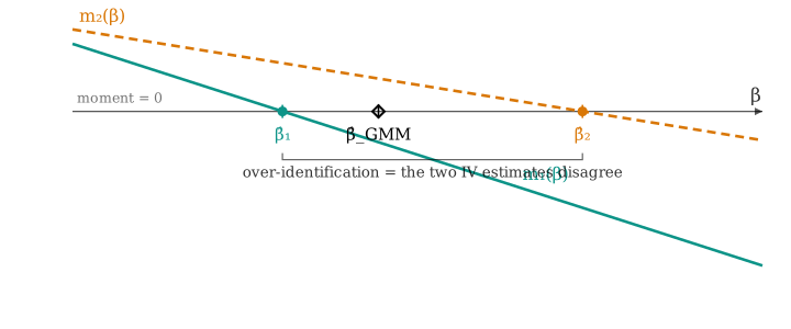
- No common zero: the two IV estimates differ, so no single \(\beta\) zeroes both moments.
- GMM compromises: minimize the weighted pair \((m_1,m_2)\); \(\bW\) sets where between \(\hat\beta_1,\hat\beta_2\).
The GMM criterion
Minimize a weighted distance of the moments
\[\boxed{\ J(\btheta)=n\,\bar{\mathbf{g}}_n(\btheta)'\,\bW\,\bar{\mathbf{g}}_n(\btheta)\ },\qquad \bW\succ0, \qquad \hat\btheta_{\text{GMM}}=\argmin_{\btheta} J(\btheta).\]
- \(\bW\) is a positive-definite weight: how much each moment (and their correlations) counts.
- Exactly identified: \(J\) reaches \(0\) at \(\bar{\mathbf{g}}_n=\bzero\) — \(\bW\) drops out (recovers MoM/IV).
- Over-identified: \(\bW\) decides how the conflicting moments are traded off — different \(\bW\), different estimator.
\(J\) has no closed form in general ⇒ numerical minimization (gancho: a otimização da Aula 13). The linear case (OLS/IV/2SLS) is the exception — \(\bar{\mathbf{g}}_n\) is linear in \(\btheta\), so \(\hat\btheta\) has a closed form (Part II).
Part II · OLS, IV and 2SLS are all GMM
Least squares
OLS is just-identified GMM
Take \(\mathbf{g}(\mathbf{d}_i,\bbeta)=\mathbf{x}_i(y_i-\mathbf{x}_i'\bbeta)\), so \(\ell=k\). The sample moment is the OLS normal equation: \[\bar{\mathbf{g}}_n(\bbeta)=\tfrac1n\bX'(\bY-\bX\bbeta)=\bzero \ \Longleftrightarrow\ \bX'\be=\bzero \ \Longrightarrow\ \hat\btheta_{\text{GMM}}=\bb_{\text{OLS}} .\]
- Exactly identified (\(\ell=k\)): \(J\) hits \(0\), weight irrelevant, GMM \(=\) OLS.
- This is the “other route” promised in Lecture 4: minimizing \(S(\mathbf{b})\) and solving the moment are the same door.
Lecture 4 split OLS into two routes — minimize the sum of squares, or solve the moment \(\bX'\be=\bzero\). GMM is the second route made general: every estimator in this course is “solve (or get as close as possible to) a moment condition.”
Instrumental variables
IV is just-identified GMM
Swap the instrument: \(\mathbf{g}=\mathbf{z}_i(y_i-\mathbf{x}_i'\bbeta)\) with \(\ell=k\). Then \[\bar{\mathbf{g}}_n(\bbeta)=\tfrac1n\bZ'(\bY-\bX\bbeta)=\bzero \ \Longrightarrow\ \hat\btheta_{\text{GMM}}=\bb_{\text{IV}}=(\bZ'\bX)^{-1}\bZ'\bY .\]
- Same recipe, instrument \(\mathbf{z}\) in place of \(\mathbf{x}\) — the Lecture 9 toolbox, now named GMM.
- Exactly identified ⇒ weight still irrelevant.
Two-stage least squares
2SLS is over-identified GMM with a specific weight
Now \(\ell>k\) with \(\mathbf{g}=\mathbf{z}_i(y_i-\mathbf{x}_i'\bbeta)\). Minimizing \(J\) with \(\bW=(\bZ'\bZ/n)^{-1}\) gives the closed form \[\hat\btheta_{\text{GMM}}(\bW)=\big(\bX'\bZ\,\bW\,\bZ'\bX\big)^{-1}\bX'\bZ\,\bW\,\bZ'\bY \ \xrightarrow{\ \bW=(\bZ'\bZ)^{-1}\ }\ \bb_{\text{2SLS}}=\big(\bX'\bP_{\bZ}\bX\big)^{-1}\bX'\bP_{\bZ}\bY .\]
- 2SLS \(=\) GMM with the particular weight \(\bW=(\bZ'\bZ)^{-1}\); substitute and \(\bP_{\bZ}=\bZ(\bZ'\bZ)^{-1}\bZ'\) appears.
- Over-identified: now the weight matters — and \((\bZ'\bZ)^{-1}\) is not generally the best one (Part III).
| Estimator | moment \(\mathbf{g}(\mathbf{d}_i,\btheta)\) | count | weight \(\bW\) |
|---|---|---|---|
| OLS | \(\mathbf{x}(y-\mathbf{x}'\bbeta)\) | \(\ell=k\) | irrelevant |
| IV | \(\mathbf{z}(y-\mathbf{x}'\bbeta)\) | \(\ell=k\) | irrelevant |
| 2SLS | \(\mathbf{z}(y-\mathbf{x}'\bbeta)\) | \(\ell>k\) | \((\bZ'\bZ)^{-1}\) |
| Efficient GMM | \(\mathbf{z}(y-\mathbf{x}'\bbeta)\) | \(\ell>k\) | \(\bS^{-1}\) (Part III) |
Part III · Efficient GMM and the optimal weight
Which weight?
Every weight is consistent — not every weight is efficient
For any fixed \(\bW\succ0\), \(\hat\btheta_{\text{GMM}}(\bW)\) is consistent (the moments are valid); \(\bW\) only changes the asymptotic variance. So: which \(\bW\) makes it smallest?
- Consistency comes from valid moments, not from the weight.
- The weight is a precision choice — the analogue of GLS vs. OLS (Lecture 7).
The optimal weight is \(\bW^{\*}=\bS^{-1}\)
With \(\bS=\Asyvar\big(\sqrt n\,\bar{\mathbf{g}}_n\big)=\E[\mathbf{g}\mathbf{g}']\) (the long-run variance of the moments), the efficient GMM weight is \(\bW^{\*}=\bS^{-1}\): \[\bS=\sigma^2\bQ_{zz}\ \text{(homosk.)}\ \Rightarrow\ \bW^{\*}=(\sigma^2\bQ_{zz})^{-1}\Rightarrow \textbf{2SLS efficient};\qquad \bS=\E[\mathbf{z}\mathbf{z}'\varepsilon^2]=\bOmega\ \text{(heterosk.)}\ \Rightarrow\ \textbf{2SLS not efficient.}\]
- Weight the moments by the inverse of their own variance — noisy moments count less.
- Homoskedastic moments: \(\bS=\sigma^2\bQ_{zz}\), and \((\bZ'\bZ)^{-1}\) matches it ⇒ 2SLS is efficient GMM.
- Heteroskedastic moments: \(\bS=\bOmega\neq\sigma^2\bQ_{zz}\) ⇒ 2SLS is beaten; efficient GMM reweights by \(\bOmega^{-1}\). This is the “efficient use of the moments” promised in Lecture 10.
Making it feasible
Feasible two-step GMM
\(\bS\) is unknown, so estimate it: \[\text{Step 1: } \bW=(\bZ'\bZ)^{-1}\ \Rightarrow\ \hat\btheta^{(1)}\ \Rightarrow\ \hat\varepsilon_i;\qquad \hat\bS=\tfrac1n\sum_i \mathbf{z}_i\mathbf{z}_i'\hat\varepsilon_i^2;\qquad \text{Step 2: } \bW=\hat\bS^{-1}\ \Rightarrow\ \hat\btheta^{(2)}.\]
- Step 1 — any valid weight gives a consistent \(\hat\btheta^{(1)}\) and residuals.
- Step 2 — reweight by \(\hat\bS^{-1}\) (heteroskedasticity-robust by construction).
- Iterated / CUE — repeat to convergence, or minimize over \(\btheta\) inside \(\bS(\btheta)\); same asymptotics.
The distribution
Asymptotic normality of GMM
With \(\bG=\E[\partial \mathbf{g}/\partial\btheta']\) (the moment Jacobian — the “bread”): \[\sqrt n\,(\hat\btheta_{\text{GMM}}-\btheta_0)\ \dto\ \Normal\!\Big(\bzero,\ (\bG'\bW\bG)^{-1}\bG'\bW\bS\bW\bG(\bG'\bW\bG)^{-1}\Big) \ \xrightarrow{\ \bW=\bS^{-1}\ }\ \Normal\!\big(\bzero,\ (\bG'\bS^{-1}\bG)^{-1}\big).\]
- A sandwich again: design inverse \(\times\) moment variance \(\times\) design inverse.
- At the optimal \(\bW=\bS^{-1}\) it collapses to \((\bG'\bS^{-1}\bG)^{-1}\) — the efficiency bound.
- Standard errors: plug in \(\hat\bG,\hat\bS\). Linear case: \(\bG=-\bQ_{zx}\) — recovers the Lecture 10 sandwich.
Part IV · Testing the overidentifying restrictions
The J-test
Overidentification test: the \(J\)-statistic
When \(\ell>k\), the surplus \(\ell-k\) moments are testable. At the efficient GMM estimate, \[J=n\,\bar{\mathbf{g}}_n(\hat\btheta)'\,\hat\bS^{-1}\,\bar{\mathbf{g}}_n(\hat\btheta)\ \dto\ \chi^2_{\ell-k} \quad\text{under } H_0:\ \E[\mathbf{g}(\mathbf{d}_i,\btheta_0)]=\bzero .\]
- The minimized criterion itself is the test statistic — \(J=J(\hat\btheta)\) at the optimal weight.
- \(=\) heteroskedasticity-robust Sargan (Lecture 10): same question, robust \(\hat\bS^{-1}\) in place of \(\sigma^2(\bZ'\bZ)^{-1}\).
- Same epistemology: tests mutual consistency of the moments; falsifies, does not confirm (shared bias passes); \(\ell=k\) ⇒ nothing to test. Reject in the upper tail.
The Lecture 10 Sargan (\(n R^2\), \(\chi^2_{\ell-k}\)) is exactly this \(J\) under homoskedastic moments. GMM gives its general, robust form — and explains why it is \(\chi^2_{\ell-k}\): \(\ell\) moments minus the \(k\) directions the estimator already forces to zero.
Part V · GMM in practice, and the bigger family
Where GMM is used
Structural vs. design-based: where GMM lives today
GMM did not fade — it split. Its place today depends entirely on which kind of empirical work you do.
- Structural economics — central. Matching model moments to data moments is GMM: demand estimation in IO (BLP), dynamic structural models, macro Euler equations, asset pricing (the SDF framework). Its simulated cousin SMM handles models with no closed-form moments.
- Design-based causal micro — receded. The credibility revolution prefers a just-identified instrument with a transparent design over efficient GMM that pools many. Why: two-step GMM’s estimated weight \(\hat\bS^{-1}\) is noisy in finite samples (bias), and over-identification trades robustness for efficiency — the wrong trade for causal work.
- Dynamic panels — with caution. Arellano–Bond / system GMM was dominant, now used carefully: instrument proliferation weakens the \(J\)-test and revives weak-IV bias.
- As theory — permanent. Even when no one “runs GMM,” OLS / IV / 2SLS / MLE are GMM (or M-estimators).
Z-estimation
Moment estimators as one family
Estimators that solve \(\tfrac1n\sum_i \boldsymbol{\psi}(\mathbf{d}_i,\btheta)=\bzero\) are Z-estimators (\(Z\) for zero). OLS, IV — and, next lecture, MLE (score \(=\bzero\)) — are all of this family; GMM extends it to the over-identified case (\(\ell>k\)).
- Just-identified: solve the moment (Z-estimator). Over-identified: minimize the weighted criterion (GMM).
- Next: MLE sets the score moment \(\E[\partial_\theta \log f]=\bzero\) — Lecture 12 as a moment estimator.
The thread continues: minimize a criterion (OLS, GMM) or solve a moment / maximize a likelihood (IV, MLE) — all extremum / M-estimators. Lecture 12 names the family and derives MLE inside it.
Summary
What to take away
- A parameter is whatever zeroes the population moments \(\E[\mathbf{g}(W,\btheta_0)]=\bzero\); estimate by the sample analogue.
- With more moments than parameters (\(\ell>k\)) you cannot zero them all — minimize the weighted criterion \(J(\btheta)=n\,\bar{\mathbf{g}}_n'\bW\bar{\mathbf{g}}_n\).
- OLS, IV and 2SLS are GMM with specific \((\mathbf{g},\bW)\) — 2SLS is GMM with \(\bW=(\bZ'\bZ)^{-1}\).
- The optimal weight is \(\bS^{-1}\) (inverse variance of the moments); it matters under heteroskedasticity, where 2SLS is no longer efficient.
- The \(J\)-test (\(\chi^2_{\ell-k}\)) is the robust Sargan: it checks the surplus moments’ mutual consistency — it falsifies, never confirms.
The original theory is Hansen (1982). In structural work GMM/SMM is standard: demand estimation (Berry et al. 1995), consumption Euler equations (Hansen and Singleton 1982), and the asset-pricing SDF framework. In dynamic panels, Arellano–Bond and system GMM (Arellano and Bond 1991) are powerful but prone to instrument proliferation (Roodman 2009). The design-based retreat reflects the finite-sample cost of the estimated optimal weight (Altonji and Segal 1996) — the Lecture 10 theme, once more.