Inference: Tests, Intervals, and the Wald Principle
Lecture 6
PIMES/UFPE
Where we are
Where this lecture sits
Lectures 4 and 5 gave us \(\bb\) and its distribution — exact under normality, asymptotically normal without it. A distribution, however, is not yet an answer. Inference turns it into statements about \(\bbeta\): is a hypothesis compatible with the data? which values are plausible? how sure can we be?
From a distribution to a decision
Three questions, one apparatus:
- Testing — is a stated value of \(\bbeta\) compatible with the data?
- Confidence — which values are not rejected? That set is the interval.
- Uncertainty — every answer carries a probability of being wrong; we control it.
Part I · Exact inference under normality
The distributions we deferred
Closing Lecture 4’s debt
Under normality the whole apparatus is exact, for every \(n\). Lecture 4 established the first piece — \(\bb\) is normal; here are the two that testing needs.
Theorem 1 (Exact sampling distributions under normality) Under A1–A4 and A6 (\(\beps \mid \bX \sim \Normal(\bzero, \sigma^2\bI_n)\)), conditional on \(\bX\):
- \(\bb \sim \Normal\!\big(\bbeta,\ \sigma^2(\bX'\bX)^{-1}\big)\);
- \(\dfrac{(n-K)\,s^2}{\sigma^2} \sim \chi^2_{\,n-K}\), and is independent of \(\bb\);
- \(\dfrac{b_k - \beta_k}{\operatorname{se}(b_k)} \sim t_{\,n-K}\), where \(\operatorname{se}(b_k) = s\sqrt{S^{kk}}\) and \(S^{kk} = [(\bX'\bX)^{-1}]_{kk}\) is the \(k\)-th diagonal element of \((\bX'\bX)^{-1}\) (Greene’s notation).
How the three distributions arise
The three in one breath: (1) a linear map of a normal is normal; (2) \((n-K)s^2 = \beps'\bM\beps\) is a quadratic form in that normal, and \(\bM\) idempotent of rank \(n-K\) makes it \(\chi^2_{n-K}\); \(\bX'\bM = \bzero\) gives the independence in (2); (3) is the normal of (1) over the root of the independent \(\chi^2\) of (2) — the unknown \(\sigma\) cancels, leaving \(s\).
Why a t, and not a normal
If \(\sigma\) were known, \((b_k-\beta_k)/(\sigma\sqrt{S^{kk}})\) would be exactly standard normal. Replacing \(\sigma\) by the estimate \(s\) injects extra uncertainty, and the price is precisely the heavier tails of the \(t_{n-K}\) — one degree of freedom lost per estimated coefficient. As \(n\) grows, \(t_{n-K} \to \Normal(0,1)\): the exact \(t\) here and the asymptotic normal of Lecture 5 are the two ends of the same object.
Confidence intervals
From the distribution to an interval
A point estimate hides its own uncertainty. We turn the distribution of \(b_k\) into a range of plausible values for \(\beta_k\). Two extremes are useless: “\(\beta_k \in b_k \pm \infty\)” is certain but empty; “\(\beta_k = b_k\) exactly” is precise but never true. We pick a confidence \(100(1-\alpha)\%\) in between.
Definition 1 (Confidence interval) Since \((b_k - \beta_k)/\operatorname{se}(b_k) \sim t_{n-K}\) (Theorem 1), this ratio lies within \(\pm t_{1-\alpha/2,\,n-K}\) with probability \(1-\alpha\); rearranging bounds \(\beta_k\). The \(100(1-\alpha)\%\) confidence interval for \(\beta_k\) is \[b_k \pm t_{1-\alpha/2,\,n-K}\,\operatorname{se}(b_k).\]
Important
The interval is random; \(\beta_k\) is fixed. “\(95\%\) confidence” is a statement about the procedure — over repeated samples, \(95\%\) of the intervals it produces contain the truth — not a probability that this one interval contains \(\beta_k\). That probability is \(0\) or \(1\); we simply do not know which.
Seeing coverage
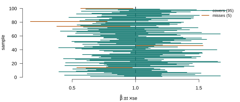
Figure 1: One hundred samples, one hundred nominal-95% confidence intervals for the same slope \(\beta=1\) (dashed). About 95 cover the truth (teal); the few that miss (amber) are the 5% we agreed to tolerate. Coverage is this repeated-sampling fact — a property of the procedure, not of any single interval.
A confidence interval for a linear combination
The same machinery covers any linear combination \(c = \mathbf{w}'\bb\) — a sum of returns, a predicted mean, a contrast. Under A6 it is normal with mean \(\mathbf{w}'\bbeta\) and variance \(\mathbf{w}'\Var[\bb\mid\bX]\,\mathbf{w}\), so \[\mathbf{w}'\bb \;\pm\; t_{1-\alpha/2,\,n-K}\,\sqrt{\mathbf{w}'\,\widehat{\Var}[\bb\mid\bX]\,\mathbf{w}}.\]
Part II · Hypothesis tests on the linear model
The testing framework
The logic, through an example
Consider a model of investment, \[\ln I_t = \beta_1 + \beta_2\,i_t + \beta_3\,\Delta p_t + \beta_4\,\ln Y_t + \beta_5\,t + \varepsilon_t,\] with \(i_t\) the nominal interest rate and \(\Delta p_t\) inflation. A rival theory says investors respond only to the real rate \(i_t - \Delta p_t\) — which is this same model under the restriction \(\beta_2 = -\beta_3\), i.e. \(\beta_2 + \beta_3 = 0\).
What a test is
A hypothesis test turns the restriction into a decision. We split the possibilities into two exclusive hypotheses — a null \(H_0\) (the restriction holds) and an alternative \(H_1\) (it does not) — and fix a rejection region: values of a test statistic so unlikely under \(H_0\) that observing them counts as evidence against it.
Size, power, and consistency
- Size \(\alpha\) — \(\Prob(\text{reject} \mid H_0 \text{ true})\): the error we choose.
- Power — \(\Prob(\text{reject} \mid H_1 \text{ true})\): the error we hope to avoid, \(1-\beta\).
- Type I: reject a true \(H_0\). Type II: fail to reject a false one.
- Consistent test — power \(\to 1\) as \(n \to \infty\): a test built on consistent estimators is itself consistent.
What “significant at 5%” does and does not say
Rejecting at \(5\%\) claims one thing: if the restriction held, data as extreme as those observed would occur in at most \(5\%\) of samples. It does not say \(H_0\) has a \(5\%\) chance of being true, nor that the effect is large, nor that it is economically relevant. Significance measures incompatibility with chance, not importance. A tiny effect is “significant” with large \(n\); a huge effect is “insignificant” with small \(n\).
The general linear restriction
A linear restriction
Every linear hypothesis — one coefficient, a difference, a sum — fits one template.
Definition 2 (Linear restriction) A set of \(J\) linear hypotheses is \(\mathbf{R}\bbeta = \mathbf{q}\), with \(\mathbf{R}\) a \(J \times K\) matrix of rank \(J\) (rows linearly independent, \(J < K\)) and \(\mathbf{q}\) a \(J\)-vector.
Take a three-coefficient model, \(\bbeta = [\,\beta_1,\ \beta_2,\ \beta_3\,]'\). Each hypothesis is one row of \(\mathbf{R}\) (picking out the right combination) set equal to an entry of \(\mathbf{q}\):
| Hypothesis | \(\mathbf{R}\) | \(\mathbf{q}\) |
|---|---|---|
| \(\beta_2 = 0\) | \([\,0\ \ 1\ \ 0\,]\) | \(0\) |
| \(\beta_1 = \beta_2\) | \([\,1\ {-1}\ \ 0\,]\) | \(0\) |
| \(\beta_2 + \beta_3 = 0\) | \([\,0\ \ 1\ \ 1\,]\) | \(0\) |
Reading off R and q
In the model \(y = \beta_0 + \beta_1 x_1 + \beta_2 x_2 + \beta_3 x_3 + \beta_4 x_4 + \beta_5 x_5 + \varepsilon\), write \(\mathbf{R}\) and \(\mathbf{q}\) for each hypothesis:
- \(\beta_3 = 0\)
- \(\beta_2 = \beta_3\)
- \(\beta_1 + \beta_2 + \beta_3 = 1\)
- \(\beta_1 = \beta_2 = \beta_3 = 0\)
- All coefficients except the intercept are zero.
Least squares under a constraint
Impose the restriction while fitting: minimize the sum of squares among the \(\bbeta\) that obey \(\mathbf{R}\bbeta = \mathbf{q}\).
Theorem 2 (Restricted least squares) The minimizer of \((\bY - \bX\bbeta)'(\bY - \bX\bbeta)\) subject to \(\mathbf{R}\bbeta = \mathbf{q}\) is \[\bb_R = \bb - (\bX'\bX)^{-1}\mathbf{R}'\big[\mathbf{R}(\bX'\bX)^{-1}\mathbf{R}'\big]^{-1}\mathbf{m}, \qquad \mathbf{m} \equiv \mathbf{R}\bb - \mathbf{q},\] where \(\bb\) is the unrestricted estimator and \(\mathbf{m}\) is the discrepancy vector — how far the unrestricted fit is from obeying the hypothesis.
Lagrangian \(S(\bbeta) + 2\boldsymbol{\lambda}'(\mathbf{R}\bbeta - \mathbf{q})\); the first-order conditions give \(\bb_R\) as \(\bb\) pulled back by exactly the amount needed to satisfy the constraint — a correction proportional to the discrepancy \(\mathbf{m}\).
Does a restriction help?
A true restriction is information: it cuts the free parameters from \(K\) to \(K-J\), and estimating fewer things from the same data is more precise.
- Under A4, exact (Greene–Seaks, 1991): \(\Var[\bb_R \mid \bX] = \Var[\bb \mid \bX] - \sigma^2(\bX'\bX)^{-1}\mathbf{R}'[\mathbf{R}(\bX'\bX)^{-1}\mathbf{R}']^{-1}\mathbf{R}(\bX'\bX)^{-1} \preceq \Var[\bb \mid \bX]\) — a psd subtraction, so \(\bb_R\) never has larger variance.
- A false restriction injects bias instead — which is what the test detects.
The clean inequality needs A4. Writing \(\bb_R - \bbeta = \mathbf{C}(\bb - \bbeta)\) with the idempotent \(\mathbf{C} = \bI - (\bX'\bX)^{-1}\mathbf{R}'[\mathbf{R}(\bX'\bX)^{-1}\mathbf{R}']^{-1}\mathbf{R}\), we get \(\Var[\bb_R\mid\bX] = \mathbf{C}\,\Var[\bb\mid\bX]\,\mathbf{C}'\). This is \(\preceq \Var[\bb\mid\bX]\) only when \(\mathbf{C}\) is an orthogonal projection in the metric of \(\Var[\bb]\) — which A4 supplies (\(\Var[\bb]=\sigma^2(\bX'\bX)^{-1}\)). Under heteroskedasticity, restricted OLS can be less precise in some directions; the estimator that always recovers the gain is restricted GLS (the efficient one, Lecture 7). The information intuition survives; only the plain-OLS identity needs A4.
Two views of the F test
Three approaches to one test
Now that \(\mathbf{R}\), \(\bb_R\) and the discrepancy \(\mathbf{m}\) are in hand, name the routes. A test compares the restricted and unrestricted fits; three ways to measure the gap, all agreeing exactly under normality (and asymptotically in general):
- Distance (Wald) — from the unrestricted fit, how far is \(\mathbf{m} = \mathbf{R}\bb - \mathbf{q}\) from \(\bzero\)?
- Fit (\(F\)) — how much does the restriction raise the residual sum of squares, \(\text{SSR}_R - \text{SSR}_U\)?
- LM (score) — from the restricted fit, how hard does it push against the constraint?
The distance view is the Wald statistic
Take the discrepancy \(\mathbf{m} = \mathbf{R}\bb - \mathbf{q}\) (from the restricted-LS slide) and ask how far it is from \(\bzero\), standardized by its own variance. That standardized distance is the Wald statistic. We build it in its exact, linear form using only normality — homoskedasticity (A4) is not needed here, and enters next only as a simplification.
Theorem 3 (The exact Wald statistic, general variance) Under \(H_0\) and A6 (normality), \(\mathbf{m}\) is normal with \(\E[\mathbf{m}\mid\bX]=\bzero\) and \(\Var[\mathbf{m}\mid\bX]=\mathbf{R}\,\Var[\bb\mid\bX]\,\mathbf{R}'\), where \(\Var[\bb\mid\bX]=\Var[\bb\mid\bX]=(\bX'\bX)^{-1}\bX'\bD\bX(\bX'\bX)^{-1}\) is the variance of \(\bb\) for a general \(\bD=\Var[\beps\mid\bX]\). Standardizing \(\mathbf{m}\) by its own variance, \[W=\mathbf{m}'\big(\mathbf{R}\Var[\bb\mid\bX]\mathbf{R}'\big)^{-1}\mathbf{m}\ \sim\ \chi^2_J\qquad(\text{exact}),\] whatever the form of \(\bD\) — only normality and the correct variance are used, not homoskedasticity.
Why \(\chi^2_J\): with \(\boldsymbol{\Sigma}=\mathbf{R}\Var[\bb\mid\bX]\mathbf{R}'\), the whitened vector \(\boldsymbol{\Sigma}^{-1/2}\mathbf{m}\sim\Normal(\bzero,\bI_J)\), so \(W=\mathbf{m}'\boldsymbol{\Sigma}^{-1}\mathbf{m}=\sum_{j=1}^J z_j^2\sim\chi^2_J\) — \(J\) standard normals, squared and summed. Sphericity of the errors is never used; only the right variance is. (But \(\Var[\bb\mid\bX]\) is unknown — the next slide makes the test feasible, and shows what estimating it costs.)
The variance is unobservable
The exact \(\chi^2_J\) above is an oracle: it divides \(\mathbf{m}\) by its true variance. That variance is unknown, and estimating it can cost the exact distribution — for two independent reasons:
| under \(H_0\) | variance known | variance estimated |
|---|---|---|
| normal errors | \(\chi^2_J\) exact | asymptotic — except A4 (next) |
| non-normal errors | asymptotic (CLT) | asymptotic (Part III) |
The variance is unknown. The exact \(\chi^2\) came from dividing \(\mathbf{m}\) by its true variance; but that variance’s core \(\bX'\bD\bX\) depends on each observation’s error size \(\sigma_i^2\), which we never see.
White’s idea. Use each point’s own squared residual \(\hat e_i^2\) as a stand-in for its \(\sigma_i^2\) — estimate the filling by \(\sum_i \hat e_i^2\,\mathbf{x}_i\mathbf{x}_i'\). The test is now computable, but we are dividing by an estimated variance, not the true one.
Why exactness is lost. Two intuitions: (i) the estimated variance is now noisy — built from residuals, it wobbles; (ii) with no A4, the numerator and the estimated variance come from the same residuals, so they move together. The clean \(\chi^2\) needed a fixed, correct variance.
What survives. With enough data the squared residuals average out to the right sizes, the estimated variance converges to the true one, and \(W\approx\chi^2_J\) — for large \(n\) only.
A4 buys back the exact distribution
The previous slide left the variance as the only obstacle to an exact test. A4 (\(\Var[\beps\mid\bX]=\sigma^2\bI\)) removes it: the sandwich collapses to a single scalar \(\sigma^2\) — and that is exactly what buys back exactness, now as an \(F\).
Corollary 1 (Classical form, the A4 special case) With \(\Var[\bb\mid\bX]=\sigma^2(\bX'\bX)^{-1}\), the variance is \(\mathbf{R}\Var[\bb\mid\bX]\mathbf{R}'=\sigma^2\mathbf{R}(\bX'\bX)^{-1}\mathbf{R}'\), so \[\underbrace{\frac{\mathbf{m}'[\mathbf{R}(\bX'\bX)^{-1}\mathbf{R}']^{-1}\mathbf{m}}{\sigma^2}}_{W\ \sim\ \chi^2_J\ (\sigma^2\text{ known})}, \qquad \underbrace{\frac{\mathbf{m}'[\mathbf{R}(\bX'\bX)^{-1}\mathbf{R}']^{-1}\mathbf{m}}{J\,s^2}}_{F\ \sim\ F_{J,\,n-K}\ (\text{exact})}.\] Unlike the robust route, here estimating the variance keeps exactness: the lone unknown \(\sigma^2\) is replaced by an independent \(s^2=\text{SSR}_U/(n-K)\) (Theorem 1, \(s^2\perp\mathbf{m}\)), turning the \(\chi^2_J\) into an exact \(F_{J,\,n-K}\).
A single coefficient: the case J = 1
The most common test is a single restriction: \(\mathbf{R} = \boldsymbol{\iota}_k'\), where \(\boldsymbol{\iota}_k\) is the \(k\)-th unit vector (the \(k\)-th column of \(\bI\): a \(1\) in slot \(k\), \(0\) elsewhere) — a row that picks out \(\beta_k\) — and \(\mathbf{q} = c\). Then \(\mathbf{m} = b_k - c\) and \(\mathbf{R}(\bX'\bX)^{-1}\mathbf{R}' = \boldsymbol{\iota}_k'(\bX'\bX)^{-1}\boldsymbol{\iota}_k = S^{kk}\), so the \(F\) is the square of a \(t\)-ratio.
Definition 3 (The t-test) For \(H_0\!: \beta_k = c\), \[t = \frac{b_k - c}{\operatorname{se}(b_k)} \sim t_{n-K}, \qquad \operatorname{se}(b_k) = s\sqrt{S^{kk}}, \qquad F = t^2 .\] Reject when \(|t| > t_{1-\alpha/2,\,n-K}\), with \(S^{kk} = [(\bX'\bX)^{-1}]_{kk}\) as above.
The familiar \(t\)-test is not a separate tool — it is the \(F\) (equivalently the Wald) for one restriction.
Large samples. Drop A6 and the exact \(t_{n-K}\) no longer holds, but the same ratio converges: \(t = (b_k - c)/\operatorname{se}(b_k) \dto \Normal(0,1)\). Both \(b_k - c\) and \(\operatorname{se}(b_k)\) are \(O_p(1/\sqrt{n})\), so the \(\sqrt{n}\) cancels — only the reference table changes (\(\Normal\) for \(t\)). With a robust \(\operatorname{se}\), this holds without A4 too.
The fit view
The distance view standardized \(\mathbf{m}\). The fit view asks the equivalent question through the residuals — and the two are literally the same number.
Because \(\bb\) is the global minimizer of the residual sum of squares \(\text{SSR}=\sum_i e_i^2\), imposing any restriction can only raise it: \[\text{SSR}_R \;\ge\; \text{SSR}_U .\]
The rise equals the standardized distance. With \(\be_* = \bY - \bX\bb_R = \be - \bX(\bb_R-\bb)\) and \(\bX'\be = \bzero\), \[\text{SSR}_R - \text{SSR}_U = (\bb_R-\bb)'\bX'\bX(\bb_R-\bb) = \mathbf{m}'[\mathbf{R}(\bX'\bX)^{-1}\mathbf{R}']^{-1}\mathbf{m},\] so the \(F\) has the equivalent fit form \[F = \frac{(\text{SSR}_R - \text{SSR}_U)/J}{\text{SSR}_U/(n-K)} = \frac{(R^2 - R^2_R)/J}{(1-R^2)/(n-K)}.\]
Joint significance is not the sum of its parts
Example 1 (Overall significance) Testing that all slopes are zero (\(H_0\!: \beta_2 = \cdots = \beta_K = 0\)) gives the “overall \(F\)” reported by every regression package, \[F = \frac{R^2/(K-1)}{(1-R^2)/(n-K)} \;\sim\; F_{K-1,\,n-K}.\] A model can have every coefficient individually insignificant yet a highly significant overall \(F\) — the hallmark of collinear regressors that are jointly, but not separately, informative.
Part III · The Wald principle
Distance-based testing
The general Wald statistic
Part II used the exact variance \(\Var[\bb\mid\bX]\) (conditional on \(\bX\)). Drop normality and that exactness goes — but the same statistic survives if we standardize by the asymptotic variance instead, estimated by \(\widehat{\Asyvar}[\bb]\) (Lecture 5).
Theorem 4 (Wald statistic) For \(H_0\!: \mathbf{R}\bbeta = \mathbf{q}\), with \(\widehat{\Asyvar}[\bb]\) a consistent estimate of the asymptotic variance of \(\bb\), \[W = (\mathbf{R}\bb - \mathbf{q})'\big[\mathbf{R}\,\widehat{\Asyvar}[\bb]\,\mathbf{R}'\big]^{-1}(\mathbf{R}\bb - \mathbf{q}) \;\dto\; \chi^2_J .\] With the classical \(\widehat{\Asyvar}[\bb] = s^2(\bX'\bX)^{-1}\) and A6 this is the Part II statistic (there with the exact \(\widehat{\Var}[\bb\mid\bX]\)), and \(W/J \sim F_{J,\,n-K}\) exactly.
Why \(\chi^2_J\) with an estimated variance. By Lecture 5, \(\sqrt{n}(\bb-\bbeta)\dto\Normal(\bzero,\bV)\) (\(\bV\) the asymptotic variance), so under \(H_0\) the distance \(\mathbf{R}\bb-\mathbf{q}\) is asymptotically normal with variance consistently estimated by \(\mathbf{R}\,\widehat{\Asyvar}[\bb]\,\mathbf{R}'\). By Slutsky the estimate replaces the truth without changing the limit: \(W\dto\chi^2_J\) — asymptotic here, exact only with a known variance (Part II).
One principle, many estimators
Every Wald test has the shape \((\text{restriction})' \,[\,\text{its variance}\,]^{-1}\, (\text{restriction})\). Change the estimator — GLS, IV, GMM (Lecture 12), maximum likelihood (Lecture 13) — and only \(\bb\) and \(\widehat{\Asyvar}[\bb]\) change; the test does not. Learning it once here is learning it for the whole course.
The Lagrange multiplier test
The restricted fit carries a Lagrange multiplier \(\boldsymbol{\lambda}_*\) on the constraint — the “pressure” the data put on it. Testing whether that pressure is zero is testing \(H_0\).
Theorem 5 (LM (score) test) With the discrepancy \(\mathbf{m} = \mathbf{R}\bb - \mathbf{q}\), \[\boldsymbol{\lambda}_* = \big[\mathbf{R}(\bX'\bX)^{-1}\mathbf{R}'\big]^{-1}\mathbf{m}, \qquad W_{LM} = \mathbf{m}'\big[\mathbf{R}\,s^2(\bX'\bX)^{-1}\mathbf{R}'\big]^{-1}\mathbf{m}.\] Since \(\boldsymbol{\lambda}_* = \bzero \iff \mathbf{R}\bbeta - \mathbf{q} = \bzero\), the LM test needs only the restricted model — and, in the linear case, no likelihood.
The score is the gradient of the fit at the restricted \(\bb_R\), namely \(\bX'\be_R\) (restricted residuals): near \(\bzero\) if \(H_0\) holds, large if not. Equivalently, it is \(nR^2\) from regressing \(\be_R\) on all regressors — the restricted fit alone, no \(\bb\) and no likelihood.
Nonlinear restrictions
When the restriction is a function
Some hypotheses are not linear in \(\bbeta\): a ratio of coefficients equal to one, a long-run multiplier, an elasticity at a point. Write them \(h(\bbeta) = \mathbf{0}\). To test them we need the distribution of \(h(\bb)\) — and \(h\) of an estimator is not, in general, normal.
The Delta Method
Theorem 6 (Delta Method) If \(\sqrt{n}(\btheta_n - \btheta) \dto \Normal(\bzero, \bV)\) (so \(\bV = \Asyvar[\btheta_n]\), the asymptotic variance) and \(h\) is continuously differentiable with Jacobian \(\bGamma = \partial h(\btheta)/\partial\btheta'\), then \[\sqrt{n}\big(h(\btheta_n) - h(\btheta)\big) \dto \Normal\!\big(\bzero,\ \bGamma\bV\bGamma'\big).\]
First-order Taylor: \(h(\btheta_n) = h(\btheta) + \bGamma(\btheta_n - \btheta) + \text{h.o.t.}\); the higher-order terms vanish in probability after rescaling by \(\sqrt{n}\), and the linear term carries the normal through. The Jacobian \(\bGamma\) is the local sensitivity (slope) of \(h\) to \(\btheta\), and it carries the variance across: \(\bV \mapsto \bGamma\bV\bGamma'\).
Nonlinear Wald
Apply the Delta Method to the restriction itself. With \(\widehat{\bGamma} = \partial h(\bbeta)/\partial\bbeta'\) evaluated at \(\bb\), \[W = h(\bb)'\big[\widehat{\bGamma}\,\widehat{\Asyvar}[\bb]\,\widehat{\bGamma}'\big]^{-1} h(\bb) \;\dto\; \chi^2_J.\] The same Wald — two substitutions from the linear case, and linear is the special case \(\bGamma=\mathbf{R}\):
| Linear | Nonlinear | |
|---|---|---|
| discrepancy | \(\mathbf{m} = \mathbf{R}\bb - \mathbf{q}\) | \(h(\bb)\) |
| variance | \(\mathbf{R}\,\widehat{\Asyvar}[\bb]\,\mathbf{R}'\) | \(\widehat{\bGamma}\,\widehat{\Asyvar}[\bb]\,\widehat{\bGamma}'\) |
Asymptotic only — the Delta Method linearizes in the limit (and \(\widehat{\bGamma},\widehat{\Asyvar}[\bb]\) are estimated), so there is no exact finite-sample analogue of the \(F\). Not invariant to how the restriction is written: \(\beta_1/\beta_2 - 1 = 0\) and \(\beta_1 - \beta_2 = 0\) are the same hypothesis but give different \(W\) in finite samples, because \(\bGamma\) changes — prefer the linear form when one exists.
Nonlinear Wald: a worked example
Example 2 (A ratio of coefficients) Test \(H_0\!:\beta_1/\beta_2=1\), i.e. \(h(\bbeta)=\beta_1/\beta_2-1=0\) (nonlinear in \(\bbeta\)). Its gradient, evaluated at \(\bb\), is the Jacobian \[\widehat{\bGamma}=\Big[\tfrac{\partial h}{\partial\beta_1},\ \tfrac{\partial h}{\partial\beta_2}\Big] =\Big[\tfrac{1}{b_2},\ -\tfrac{b_1}{b_2^{2}}\Big].\]
Under \(H_0\) the Delta Method makes the restriction asymptotically normal — \(h(\bb)\) is approximately \(\Normal\!\big(0,\ \widehat{\bGamma}\,\widehat{\Asyvar}[\bb]\,\widehat{\bGamma}'\big)\) — so standardizing gives the (\(J=1\)) Wald statistic \[W=\frac{h(\bb)^2}{\widehat{\bGamma}\,\widehat{\Asyvar}[\bb]\,\widehat{\bGamma}'}\ \dto\ \chi^2_1.\] The denominator is the Delta-Method variance of the ratio; its square root is \(\operatorname{se}(h(\bb))\).
The ratio test, by the numbers
Suppose \(b_1=2\), \(b_2=1\), with estimated variance \[\widehat{\Asyvar}[\bb]=\begin{bmatrix}0.09 & 0.02\\[2pt] 0.02 & 0.04\end{bmatrix} \quad(\operatorname{se}(b_1)=0.3,\ \operatorname{se}(b_2)=0.2,\ \widehat{\Cov}=0.02).\]
- Restriction: \(h(\bb)=b_1/b_2-1=2/1-1=1\).
- Jacobian: \(\widehat{\bGamma}=[\,1/b_2,\ -b_1/b_2^2\,]=[\,1,\ -2\,]\).
- Variance of \(h(\bb)\) (Delta): \[\widehat{\bGamma}\,\widehat{\Asyvar}[\bb]\,\widehat{\bGamma}' =\underbrace{1^2(0.09)+(-2)^2(0.04)}_{0.25}+\underbrace{2\,(1)(-2)(0.02)}_{-0.08}=0.17,\] so \(\operatorname{se}(h(\bb))=\sqrt{0.17}=0.412\) — the covariance term \((-0.08)\) is not optional.
- Statistic: \(W=h(\bb)^2/0.17=1/0.17=5.88\).
- Decision: \(\chi^2_{1,\,0.95}=3.84\); since \(5.88>3.84\), reject \(H_0:\beta_1/\beta_2=1\) at \(5\%\) (equivalently \(z=\sqrt{W}=2.43\), \(p\approx0.015\)).
The Wald statistic, in general
One statistic across three axes: everything in Part III was the same distance, weighted by its own variance. Now that each axis has been developed, the summary:
| Axis | Part II (exact) | Wald, in general |
|---|---|---|
| Variance | exact \(\Var[\bb\mid\bX]\) (A4 \(\Rightarrow\) classical) | asymptotic \(\widehat{\Asyvar}[\bb]\) (any consistent; robust sandwich) |
| Sample | exact \(F\)/\(\chi^2\) under A6 | asymptotic \(\chi^2_J\) without A6 |
| Restriction | linear \(\mathbf{R}\bb-\mathbf{q}\) | nonlinear \(h(\bb)\) via the Delta Method |
Part IV · Joint inference and stability
Joint versus marginal
Two intervals are not a region
Testing \(\beta_1\) and \(\beta_2\) separately is not testing them jointly. Because \(b_1\) and \(b_2\) are correlated, the joint \(95\%\) region is an ellipse, not the rectangle formed by the two marginal intervals.
- A point can lie inside both marginal intervals yet outside the joint region — and vice versa.
- Two \(5\%\) tests do not make a \(5\%\) joint test: the error rates compound.
- The tilt of the ellipse is the correlation of the estimators.
Seeing the confidence ellipse
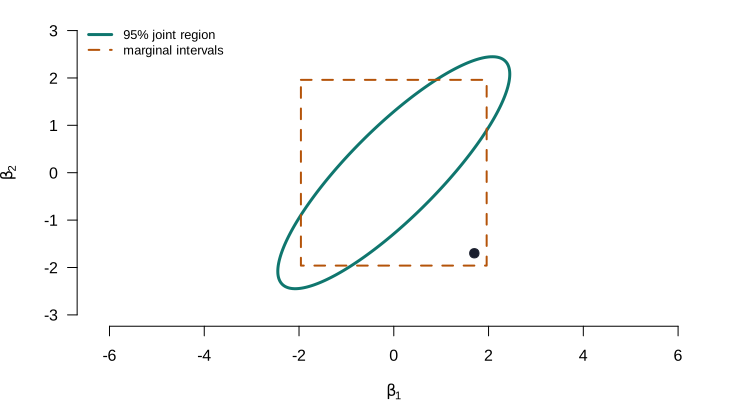
Figure 2: A 95% joint confidence region (ellipse) for correlated \((\beta_1,\beta_2)\), and the box of the two marginal 95% intervals. The dot is inside both marginal intervals yet outside the joint region: two separate tests are not one joint test.
Structural stability
Has the relationship changed?
Did the 1973 oil shock change the structure of the U.S. gasoline market? Split the sample at 1973 and let each period have its own coefficients — the unrestricted model is block-diagonal, \(\mathbf{y} = \operatorname{diag}(\bX_1, \bX_2)(\bbeta_1', \bbeta_2')' + \beps\), which is just OLS on each subsample. “No structural break” is the restriction \(\bbeta_1 = \bbeta_2\), i.e. \(\mathbf{R} = [\bI : -\bI]\), \(\mathbf{q} = \bzero\) — and imposing it is OLS on the pooled data.
Example 3 (The Chow test) Under \(H_0\!:\bbeta_1 = \bbeta_2\), with \(\be_1, \be_2\) the separate residuals and \(\be_*\) the pooled, \[F = \frac{\big(\be_*'\be_* - (\be_1'\be_1 + \be_2'\be_2)\big)/K}{(\be_1'\be_1 + \be_2'\be_2)/(n_1 + n_2 - 2K)} \sim F_{K,\,n_1+n_2-2K}.\] An ordinary \(F\): the pooled fit is the restricted model, the two separate fits the unrestricted one.
What we have, and where it goes
The scoreboard
| Exact (finite sample) | Large sample | |
|---|---|---|
| Needs | A6 (normal errors) | no A6; A5a, A2\('\) |
| One coefficient | \(t_{n-K}\) | \(\Normal(0,1)\) |
| \(J\) restrictions | \(F_{J,\,n-K}\) | \(\chi^2_J\) (Wald) |
| Variance used | classical \(s^2(\bX'\bX)^{-1}\) | robust sandwich |
| Nonlinear \(h(\bbeta)\) | — | Delta Method + Wald |
Reading
Sources
| Hansen | Chapter 8 (restricted estimation) and Chapter 9 (hypothesis testing, Wald and the \(F\)-test) |
| Greene | Chapter 5 (hypothesis tests and model selection; interval estimation and prediction) |