Conditional Expectation, Linear Projection, and the Linear Regression Model
Lecture 2
PIMES/UFPE
Before any model
Where this lecture sits
This lecture answers the first of the three questions, and only that one. By the end we will know under exactly what conditions the parameter of a linear model can be learned from data — and we will not have written down a single estimator. Estimation is Lecture 3; inference waits until Lecture 6.
The question of this lecture
We observe a sample and want to say something about the relationship between \(y\) and \(\mathbf{x}\). The instinct is to write down a model. Resist it for a moment, and ask instead: what can be said before assuming anything at all?
\(\{(y_i, \mathbf{x}_i)\}_{i=1}^n\) are i.i.d. draws from a population distribution \(F\), with \(y_i\) scalar and \(\mathbf{x}_i\) a \(K \times 1\) vector.
That is the entire assumption. No linearity, no exogeneity, no functional form.
Notation, once and for all
Every vector and matrix used in this course is fixed here, so that no later slide has to stop and explain a shape.
A single observation pairs a scalar \(y_i\) with a \(K \times 1\) vector of regressors, and a coefficient vector has the same length:
\[\underset{K \times 1}{\mathbf{x}_i} = \begin{pmatrix} x_{i1} \\ x_{i2} \\ \vdots \\ x_{iK}\end{pmatrix}, \qquad \underset{K \times 1}{\bbeta} = \begin{pmatrix} \beta_1 \\ \beta_2 \\ \vdots \\ \beta_K \end{pmatrix}, \qquad \mathbf{x}_i'\bbeta = \sum_{k=1}^{K} x_{ik}\beta_k \quad (1 \times 1).\]
Ordinarily \(x_{i1} = 1\), the constant. Note that \(\mathbf{x}_i'\bbeta\) is a scalar — the most common slip at this stage is to read it as a matrix.
Stacking the sample
Stacking the \(n\) observations gives the form used for the rest of the course:
\[\underset{n \times 1}{\bY} = \underset{n \times K}{\bX}\;\underset{K \times 1}{\bbeta} + \underset{n \times 1}{\beps}, \qquad \bX = \begin{pmatrix} \mathbf{x}_1' \\ \mathbf{x}_2' \\ \vdots \\ \mathbf{x}_n' \end{pmatrix}.\]
Throughout, \(i\) indexes rows, meaning observations, and \(k\) indexes columns, meaning variables. Boldface lower case is a vector, boldface upper case a matrix.
Two population moments
Two averages of these objects will appear repeatedly from the middle of the lecture onward:
\[\underset{K \times K}{\bQ_{xx}} = \E[\mathbf{x}\mathbf{x}'] = \begin{pmatrix} \E[x_1^2] & \E[x_1x_2] & \cdots & \E[x_1x_K] \\ \E[x_2x_1] & \E[x_2^2] & \cdots & \E[x_2x_K] \\ \vdots & \vdots & \ddots & \vdots \\ \E[x_Kx_1] & \E[x_Kx_2] & \cdots & \E[x_K^2] \end{pmatrix}, \qquad \underset{K \times 1}{\E[\mathbf{x}y]} = \begin{pmatrix} \E[x_1y] \\ \E[x_2y] \\ \vdots \\ \E[x_Ky] \end{pmatrix}.\]
\(\bQ_{xx}\) is symmetric, since \(\E[x_jx_k] = \E[x_kx_j]\). Both are features of the population, not of any sample: no \(i\) appears in either.
Two objects, and why the order matters
It turns out that a joint distribution alone gives us two well-defined objects: the conditional expectation function, which describes the average of \(y\) at each value of \(\mathbf{x}\), and the linear projection, which is the best straight-line summary of that relationship. Neither requires a model. Both exist as soon as a few moments are finite.
Only afterwards do we impose the linear regression model — and the model turns out to be precisely the assumption that these two objects coincide.
The conditional expectation function
What we actually want to know
The interest is always conditional. Start with a single binary indicator.
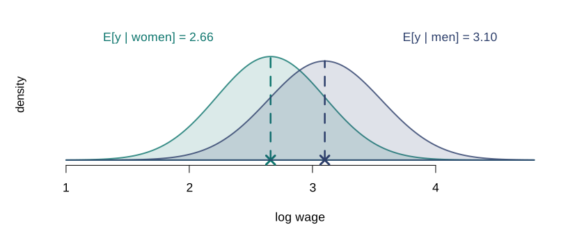
Figure 1: Log wages for two groups. The dashed segments mark the group means — and that pair of numbers is the conditional expectation function.
The definition
Definition 1 (Conditional expectation function) The conditional expectation function (CEF) is \[m(\mathbf{x}) = \E[y \mid \mathbf{x}],\] the mean of \(y\) in the subpopulation with covariates equal to \(\mathbf{x}\). It exists whenever \(\E|y| < \infty\), and involves no modelling assumption whatever.
With one binary regressor, \(m\) takes two values. With two binary regressors it takes four. As the conditioning becomes finer the CEF becomes a richer object — and with a continuous regressor it becomes a curve.
More groups, same idea
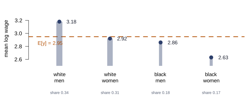
Figure 2: Mean log wage in four groups defined by sex and race; stem width is proportional to the group’s population share. The dashed line is the unconditional mean. Note the vertical axis does not start at zero.
The law of iterated expectations, read off the figure
The dashed line is the unconditional mean, and it is not the average of the four bars. It is their average weighted by the group shares:
\[\E[y] \;=\; \sum_{g} \Prob(\text{group } g)\; \E[y \mid \text{group } g]\]
which is exactly the law of iterated expectations, \(\E[y] = \E\big[\E[y \mid \mathbf{x}]\big]\). The outer expectation averages the group means over the distribution of the groups.
The CEF error
Whatever \(m\) is, we can define the deviation of \(y\) from it: write \(\varepsilon = y - m(\mathbf{x})\), so that \(y = m(\mathbf{x}) + \varepsilon\).
Theorem 1 (Properties of the CEF error)
- \(\E[\varepsilon \mid \mathbf{x}] = 0\)
- \(\E[\varepsilon] = 0\)
- \(\E[h(\mathbf{x})\,\varepsilon] = 0\) for any \(h\) with \(\E|h(\mathbf{x})\varepsilon| < \infty\)
Proof.
- holds because \(m(\mathbf{x})\) is a function of \(\mathbf{x}\), so it passes through the conditional expectation. (2) is (1) plus the law of iterated expectations. (3) follows by conditioning on \(\mathbf{x}\) first, which reduces the expression to \(\E[h(\mathbf{x}) \cdot 0]\). \(\square\)
Nothing here has been assumed
Read the theorem again and notice what it is not. The equation \(y = m(\mathbf{x}) + \varepsilon\) with \(\E[\varepsilon \mid \mathbf{x}] = 0\) holds by construction, for any joint distribution with a finite mean. It has no empirical content: nothing has been assumed, and consequently nothing can be tested.
Why the mean, and not something else?
Among all functions of \(\mathbf{x}\), the CEF predicts \(y\) best under squared loss.
Theorem 2 (The CEF minimises mean squared error) Among all \(g\) with \(\E[g(\mathbf{x})^2] < \infty\), \[m(\mathbf{x}) = \argmin_{g} \E\big[(y - g(\mathbf{x}))^2\big].\]
Proof. Add and subtract \(m(\mathbf{x})\) inside the square. The cross term vanishes by Theorem 1(3), since \(m - g\) is a function of \(\mathbf{x}\), leaving \[\E\big[(y - g(\mathbf{x}))^2\big] = \E[\varepsilon^2] + \E\big[(m(\mathbf{x}) - g(\mathbf{x}))^2\big] \ge \E[\varepsilon^2],\] with equality only when \(g\) and \(m\) agree as functions of \(\mathbf{x}\). \(\square\)
Conditional variance
The mean is not the only thing that moves
The CEF records the centre of each conditional distribution and discards everything else. Some of what it discards matters.
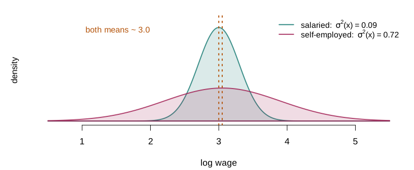
Figure 3: Two groups with essentially the same conditional mean and very different conditional variance. The CEF cannot tell them apart.
Naming what the CEF leaves out
What the figure shows is dispersion in \(y\) within each group. That is the object to name, and we name it on \(y\) — the same variable the CEF was about.
Definition 2 (Conditional variance) The conditional variance of \(y\) given \(\mathbf{x}\) is \[\sigma^2(\mathbf{x}) \;=\; \Var[y \mid \mathbf{x}] \;=\; \E\big[(y - m(\mathbf{x}))^2 \bigm| \mathbf{x}\big].\]
The same object, read on the error
The bracket in Definition 2 is \(\varepsilon^2\), since \(\varepsilon = y - m(\mathbf{x})\). So the conditional variance can be written three ways:
\[\sigma^2(\mathbf{x}) \;=\; \Var[y \mid \mathbf{x}] \;=\; \Var[\varepsilon \mid \mathbf{x}] \;=\; \E[\varepsilon^2 \mid \mathbf{x}].\]
- Given \(\mathbf{x}\), the number \(m(\mathbf{x})\) is fixed — subtracting it shifts the distribution without changing its spread
- \(\E[\varepsilon \mid \mathbf{x}] = 0\) by construction kills the squared-mean term
One object, not two. We write it on the error, because that is the form Lecture 4 needs.
Conditional and unconditional are different objects
The unconditional variance \(\sigma^2 = \E[\varepsilon^2]\) is a single number. The conditional variance \(\sigma^2(\mathbf{x})\) is a function. They are linked, again, by iterated expectations:
\[\sigma^2 \;=\; \E\big[\sigma^2(\mathbf{x})\big]\]
so the unconditional variance is the average of the conditional ones. Knowing \(\sigma^2\) tells you nothing about how the spread varies across groups — exactly as knowing \(\E[y]\) told you nothing about the four group means.
Definition 3 (Homoskedasticity and heteroskedasticity) The conditional variance is homoskedastic if \(\sigma^2(\mathbf{x}) = \sigma^2\) does not depend on \(\mathbf{x}\), and heteroskedastic otherwise.
Which case is the exception?
Important
Textbooks often present homoskedasticity as part of a correct specification and heteroskedasticity as a deviation from it. That is backwards.
Heteroskedasticity is the generic case; homoskedasticity is unusual and exceptional. The default in empirical work should be to assume the errors are heteroskedastic, not the converse.
Would you expect the dispersion of wages to be the same for those with 4 and with 16 years of schooling? Nobody expects that. Constant variance is a coincidence — and coincidences should not be the default.
When the CEF is linear
The convenient special case
We have a target, \(m(\mathbf{x})\), and no way to estimate a whole function. The obvious question is when \(m\) happens to be simple enough to estimate.
Definition 4 (Linear CEF) The CEF is linear if \[m(\mathbf{x}) = \E[y \mid \mathbf{x}] = \mathbf{x}'\bbeta\] for some \(K\)-vector \(\bbeta\), where \(\mathbf{x}\) ordinarily includes a constant.
When this holds, the object we wanted is described by \(K\) numbers, and estimating it becomes feasible. Everything the rest of the course does to the linear model rests on this being either true or a good enough approximation.
Linearity is less restrictive than it looks
With discrete regressors it is not an assumption at all. Take the four groups of Figure 2 and include a constant plus three dummies. Four parameters, four group means: the linear CEF fits them exactly, whatever the numbers happen to be. A saturated regression on dummies is always a linear CEF.
Linear in parameters, not in variables. \(\mathbf{x}\) may contain \(x^2\), \(\log x\), interactions or splines. Writing \(m(x) = \beta_1 + \beta_2 x + \beta_3 x^2\) is a linear CEF in a nonlinear function of \(x\) — and by adding terms one can approximate a curve as closely as desired.
And when it is not linear?
Nothing guarantees the CEF is linear, and with continuous regressors it usually is not. Two responses are available.
One is to estimate \(m\) without restricting its shape. That is nonparametric regression, it works, and it needs far more data than economics usually has — the reason being precisely the infinite-dimensional minimisation of Theorem 2.
The other is to keep the linear form and ask what, exactly, we get: if we insist on a linear function anyway, which one do we get, and does it mean anything? That object occupies the rest of this lecture.
Linear projection
The best linear approximation
We give up on describing \(m\) exactly. Instead of the best predictor among all functions of \(\mathbf{x}\), ask for the best predictor among the linear ones — the coefficient vector that makes \(\mathbf{x}'\mathbf{c}\) as close to \(y\) as possible, under the same squared loss.
Minimising over \(K\) numbers instead of a function
Definition 5 (Linear projection) Suppose \(\E[y^2] < \infty\), \(\E\|\mathbf{x}\|^2 < \infty\), and \(\bQ_{xx} = \E[\mathbf{x}\mathbf{x}']\) is nonsingular. The linear projection coefficient is \[\bbeta = \argmin_{\mathbf{c}\,\in\,\mathbb{R}^K} S(\mathbf{c}), \qquad S(\mathbf{c}) = \E\big[(y - \mathbf{x}'\mathbf{c})^2\big],\] and the linear projection of \(y\) on \(\mathbf{x}\) is \(\mathbf{x}'\bbeta\).
Here \(\mathbf{c}\) ranges over candidate coefficient vectors and \(\bbeta\) is the one that wins. Both are features of the distribution \(F\): no data appears anywhere in Definition 5, and none will until Lecture 3.
The closed form
Theorem 3 (The projection coefficient) Under the conditions of Definition 5, \[\bbeta = \bQ_{xx}^{-1}\,\E[\mathbf{x}y].\]
Proof. Expanding the square and taking expectations, \(S(\mathbf{c}) = \E[y^2] - 2\,\mathbf{c}'\E[\mathbf{x}y] + \mathbf{c}'\bQ_{xx}\mathbf{c}\), a quadratic form in \(\mathbf{c}\). Its first-order condition is \[\frac{\partial S}{\partial \mathbf{c}} = -2\,\E[\mathbf{x}y] + 2\,\bQ_{xx}\mathbf{c} = \bzero,\] which has the unique solution \(\bQ_{xx}^{-1}\E[\mathbf{x}y]\) because \(\bQ_{xx}\) is nonsingular, and is a minimum because the Hessian \(2\bQ_{xx}\) is positive definite. \(\square\)
The formula in the simplest case
The formula is worth cashing out once by hand. With a constant and one regressor, \(\mathbf{x} = (1, x_2)'\), the two moments are small enough to invert:
\[\bQ_{xx} = \begin{pmatrix} 1 & \E[x_2] \\ \E[x_2] & \E[x_2^2] \end{pmatrix}, \qquad \E[\mathbf{x}y] = \begin{pmatrix} \E[y] \\ \E[x_2y] \end{pmatrix},\]
and carrying out \(\bQ_{xx}^{-1}\E[\mathbf{x}y]\) gives
\[\beta_2 = \frac{\E[x_2y] - \E[x_2]\,\E[y]}{\E[x_2^2] - \E[x_2]^2} = \frac{\Cov(x_2,y)}{\Var(x_2)}, \qquad \beta_1 = \E[y] - \beta_2\,\E[x_2].\]
The population regression slope, in the form every introductory course states it — and here \(\det \bQ_{xx} = \Var(x_2)\), so “nonsingular” just means the regressor varies.
What the formula buys
Definition 5 says what \(\bbeta\) is. Theorem 3 says what it equals.
Reading \(\bbeta = \bQ_{xx}^{-1}\E[\mathbf{x}y]\), all it needs is
- two finite moments, and
- \(\bQ_{xx}\) invertible.
No linear CEF. No true model. No model at all — and the solution is unique.
The projection error
Define the projection error \(e = y - \mathbf{x}'\bbeta\), so that
\[y = \mathbf{x}'\bbeta + e\]
holds by construction — exactly as \(y = m(\mathbf{x}) + \varepsilon\) did. Rewriting the first-order condition of Theorem 3 in terms of \(e\) gives \(K\) equations:
\[\E[\mathbf{x}e] = \bzero.\]
What those \(K\) equations say
Take the first regressor to be the constant, \(x_1 = 1\). Then the first of the \(K\) equations reads \(\E[e] = 0\), and each of the others, \(\E[x_ke] = 0\), combines with it to give
\[\Cov(x_k, e) = \E[x_ke] - \E[x_k]\,\E[e] = 0, \qquad k = 2,\dots,K.\]
So the whole content of “this is the best line” is:
Important
The projection error is uncorrelated with each regressor. That is all.
Minimising \(S(\mathbf{c})\) buys zero correlation and nothing else — no statement about the error at any particular value of \(\mathbf{x}\).
And what the CEF error satisfies instead
The CEF error obeys something visibly stronger:
\[\E[\varepsilon \mid \mathbf{x}] = 0 \quad\text{for every value of } \mathbf{x}.\]
This is mean independence: the average error is zero not on average overall, but separately within every subpopulation. Mean independence implies zero correlation; the converse fails. Two conditions, then, and it is worth fixing the names now because the rest of the lecture turns on the difference.
| Condition | Holds for | |
|---|---|---|
| Zero correlation | \(\Cov(x_k, e) = 0\), i.e. \(\E[\mathbf{x}e] = \bzero\) | the projection error, always |
| Mean independence | \(\E[\varepsilon \mid \mathbf{x}] = 0\) | the CEF error, always |
The second implies the first. The first does not imply the second.
The two errors, compared
We now have two decompositions of the same \(y\):
\[y = m(\mathbf{x}) + \varepsilon \qquad\text{and}\qquad y = \mathbf{x}'\bbeta + e.\]
The left-hand sides agree, so the right-hand sides must too. Solving for \(e\):
\[e \;=\; \varepsilon \;+\; \underbrace{\big[\,m(\mathbf{x}) - \mathbf{x}'\bbeta\,\big]}_{\text{approximation error}}\]
The projection error is the CEF error plus the amount by which the best line misses the CEF.
The gap between the two conditions
Take conditional expectations of that decomposition. The first term dies by construction; the second is a function of \(\mathbf{x}\), so conditioning on \(\mathbf{x}\) leaves it untouched:
\[\E[e \mid \mathbf{x}] \;=\; \underbrace{\E[\varepsilon \mid \mathbf{x}]}_{=\;0} \;+\; m(\mathbf{x}) - \mathbf{x}'\bbeta \;=\; m(\mathbf{x}) - \mathbf{x}'\bbeta.\]
So \(\E[e \mid \mathbf{x}]\) is the approximation error — and that identity answers the question of how the two conditions relate:
- the projection error satisfies zero correlation always, by construction;
- it satisfies mean independence only when the approximation error is identically zero — that is, only when the CEF is linear, in which case \(e = \varepsilon\).
Seeing the gap
The true CEF here is quadratic; the projection is the best line through it. The vertical distance between the two curves is the approximation error \(m(x) - \mathbf{x}'\bbeta\).
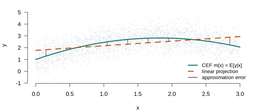
Figure 4: A nonlinear CEF (solid) and its linear projection (dashed). The vertical segments are the approximation error.
The two conditions, on one set of axes
Now plot the projection errors themselves, and put both conditions on the same picture.
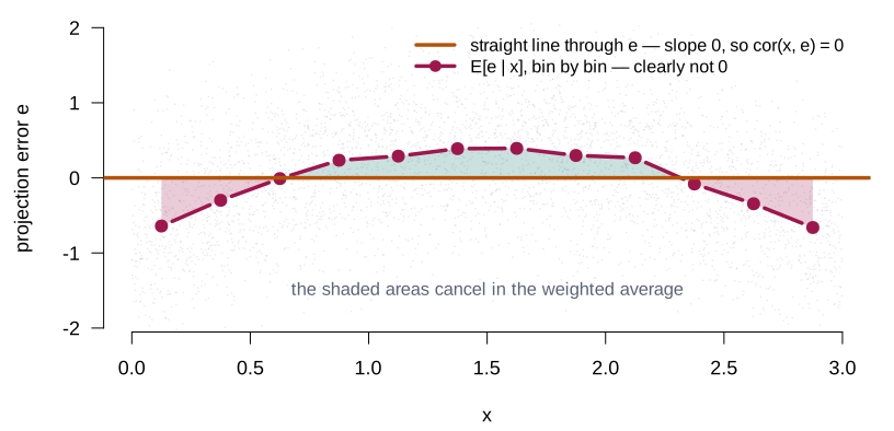
Figure 5: The same projection errors, with both conditions drawn on them. The straight line through the errors is flat — zero correlation holds. The conditional mean of the errors is not flat — mean independence fails. The shaded areas are what cancel.
Why one is flat and the other is not
The straight line is flat because zero correlation forces it to be: fitting a line to \(e\) against \(x\) recovers the slope \(\Cov(x,e)/\Var(x)\), and that numerator is zero by construction.
The curve is not flat because nothing forces it to be. It is \(\E[e \mid x]\), which the previous section identified as the approximation error — negative where the line sits above the CEF, positive where it sits below.
Important
The two are consistent because the negative stretches and the positive stretch cancel when averaged over the distribution of \(x\).
Zero correlation constrains that one weighted average, once per regressor. Mean independence would constrain the crimson curve to sit on zero at every \(x\).
A small equation with a long future
\(\E[\mathbf{x}e] = \bzero\) is a moment condition — a statement that some function of the data and the parameter has mean zero. Follow it forward:
- Lecture 3 — its sample analogue \(\bX'\be = \bzero\) drops out of least squares algebra
- Lecture 10 — the regressor is replaced by an instrument, giving \(\E[\mathbf{z}e] = \bzero\)
- Lecture 12 — it generalises to \(\E[g(W,\btheta)] = \bzero\), which is GMM
The linear regression model
Nothing new from here
It is worth pausing to record how little has been assumed. The CEF exists whenever \(y\) has a mean. The projection exists whenever two moments are finite and \(\bQ_{xx}\) inverts. Both decompositions of \(y\) hold by construction. Nothing in this lecture so far could be contradicted by data.
The linear regression model is the single statement that ties the two objects together:
\[y = \mathbf{x}'\bbeta + \varepsilon, \qquad \E[\varepsilon \mid \mathbf{x}] = 0.\]
This is Definition 4, and it is worth checking that the equivalence really runs both ways.
The equivalence, both directions
If the CEF is linear, set \(\varepsilon = y - m(\mathbf{x}) = y - \mathbf{x}'\bbeta\). This is the CEF error, so \(\E[\varepsilon \mid \mathbf{x}] = 0\) by construction, and the display holds.
Conversely, suppose the display holds. Take \(\E[\,\cdot \mid \mathbf{x}]\) of both sides: \[\E[y \mid \mathbf{x}] = \mathbf{x}'\bbeta + \E[\varepsilon \mid \mathbf{x}] = \mathbf{x}'\bbeta,\] which says the CEF is linear.
So “the CEF is linear” and “the error is mean independent of \(\mathbf{x}\)” are the same assumption stated two ways — and, by the comparison of the two errors, it is also the assumption that the approximation error is identically zero.
Three names for what we already have
The three conditions below are the ones Lectures 3 and 4 refer to by name. None of them is new material: each is something already established, given a label so it can be pointed at individually.
| Where it came from | |
|---|---|
| A1 Linearity | Definition 4 — the CEF is \(\mathbf{x}'\bbeta\) |
| A2 Full rank | Definition 5 — \(\bQ_{xx}\) nonsingular |
| A3 Exogeneity | the comparison of the two errors |
A1 · Linearity
\[m(\mathbf{x}) = \E[y \mid \mathbf{x}] = \mathbf{x}'\bbeta\]
This is Definition 4. Its consequence is the one the lecture has been working towards: the approximation error \(m(\mathbf{x}) - \mathbf{x}'\bbeta\) is identically zero, the projection coefficient and the CEF coefficient are the same vector, and \(\bbeta\) is a derivative of a conditional mean rather than the slope of an approximating line.
Linearity remains in the parameters: \(x^2\), \(\log x\) and interactions are all allowed.
A2 · Full rank, and why it is about identification
\[\bQ_{xx} = \E[\mathbf{x}\mathbf{x}'] \ \text{nonsingular}; \qquad \text{in the sample, } \rank(\bX) = K \ \text{with } n \ge K.\]
This is the condition Definition 5 already required, now named. Its sample counterpart is what makes \(\bX'\bX\) invertible in Lecture 3. It is tempting to read it as a technical convenience that makes a formula work. It is not.
Important
If A2 fails, distinct values of \(\bbeta\) produce identical distributions of the observables. No estimator can tell them apart, at any sample size. This is an identification failure, not a computational one.
What that looks like
Example 1 (An unestimable model) \[\ln \text{Price} = \beta_1 \ln \text{Size} + \beta_2 \ln \text{AspectRatio} + \beta_3 \ln \text{Height} + \varepsilon\]
with \(\text{Size} = W \times H\) and \(\text{AspectRatio} = W/H\). Then \(\ln\text{Size} = \ln W + \ln H\) and \(\ln\text{AspectRatio} = \ln W - \ln H\), so \[\ln\text{Size} - \ln\text{AspectRatio} - 2\ln H = 0\] exactly. The three regressors are collinear, each \(\beta_k\) is meaningless on its own, and only certain linear combinations are identified.
A3 · Exogeneity
\[\E[\varepsilon \mid \mathbf{x}] = 0, \qquad \text{stacked: } \E[\beps \mid \bX] = \bzero.\]
This is the strengthening of \(\E[\mathbf{x}e] = \bzero\) that the comparison of the two errors isolated. The projection always delivers zero correlation; A3 asks for zero conditional mean, which is the same as asking that the approximation error be zero everywhere.
So A1 and A3 are not independent statements — given A1, the error of the linear specification is a CEF error and A3 follows. They are separated only because they fail for different reasons and are repaired by different techniques: a wrong functional form is one problem, an omitted variable is another.
Where exogeneity fails
Example 2 (Omitted variables) Suppose the DGP is \(\text{Income} = \gamma_1 + \gamma_2\,\text{educ} + \gamma_3\,\text{age} + u\) but we estimate \(\text{Income} = \gamma_1 + \gamma_2\,\text{educ} + \varepsilon\).
Then \(\varepsilon = \gamma_3\,\text{age} + u\), so \(\E[\varepsilon \mid \text{educ}] = \gamma_3\,\E[\text{age} \mid \text{educ}] \neq 0\) whenever age and education are related.
A3 fails here, and the failure is not a technicality: it is omitted variable bias, which we derive properly in Lecture 4 and spend Lectures 10 and 11 learning to repair.
What each condition buys
| Restricts | Buys | Revisited in | |
|---|---|---|---|
| A1 Linearity | the shape of \(m(\mathbf{x})\) | \(\bbeta\) is a CEF coefficient | Lectures 13–14 |
| A2 Full rank | \(\bQ_{xx}\) | Identification; \((\bX'\bX)^{-1}\) exists | Lecture 3 |
| A3 Exogeneity | \(\varepsilon\) given \(\mathbf{x}\) | Unbiasedness, consistency | Lectures 10–11 |
The model as stated says nothing about the conditional variance, and nothing about the shape of the conditional distribution. Those are separate restrictions, and they enter later — in Lecture 4, where each is first needed for a result that cannot be had without it.
Identification, before estimation
Putting the pieces together
We now have everything needed to answer the first of the three questions from Lecture 1, and notice that we have not yet written down a single estimator.
The parameter \(\bbeta\) is a functional of the population moments, \(\bbeta = \bQ_{xx}^{-1}\E[\mathbf{x}y]\). It is therefore determined by \(F\) alone — provided \(\bQ_{xx}\) can be inverted. A2 delivers exactly that: given A2, no two values of \(\bbeta\) generate the same joint distribution, and the parameter is identified.
Two conditions, two jobs
A3 does a separate job, and it is about what the identified vector means.
What A3 adds
Without A3, \(\bbeta\) is identified but \(\mathbf{x}'\bbeta\) is only the best straight-line approximation to the CEF: the two differ by the approximation error. With A3 that error is zero, so
\[\mathbf{x}'\bbeta = \E[y \mid \mathbf{x}],\]
and the line we identified is the conditional expectation function rather than an approximation to it. That is what licenses reading \(\beta_k\) as the effect of \(x_k\) on the average of \(y\).
Important
A2 identifies \(\bbeta\). A3 makes \(\bbeta\) the thing we wanted.
Two different jobs, failing for two different reasons, repaired by two different techniques.
Estimation is next lecture — and, as we will see, it is by some distance the easier problem.
Reading
Sources
| Hansen (Hansen 2022) | Chapter 2 — the CEF, conditional variance, the linear CEF, and projection |
| Greene (Greene 2018) | Chapter 2 — the two examples used here |