Properties of IV, Weak Instruments, and Specification Tests
Lecture 10
PIMES/UFPE
Where we are
Where this lecture sits
Lecture 9 restored consistency under endogeneity — a valid instrument recovers the structural \(\bbeta\) that OLS misses. Now the bill: at what price? Three prices, the honest accounting after any IV estimate:
- Less precise than OLS — using only the instrumented slice of \(\mathbf{x}\) costs variance.
- Fragile under a weak instrument — a first stage that barely moves \(\mathbf{x}\) breaks finite-sample guarantees.
- Only partly testable — endogeneity and overidentification can be probed; exclusion stays a design argument.
Part I · The price of IV: variance and efficiency
The asymptotic distribution
What 2SLS converges to
Under relevance (full-rank \(\bQ_{zx}=\E[\mathbf{z}\mathbf{x}']\)), exogeneity, and finite moments, scale the 2SLS error by \(\sqrt n\) and read off a bread–meat sandwich — a design inverse around a score variance: \[\sqrt n\,(\bb_{\text{2SLS}}-\bbeta)=\underbrace{\Big(\tfrac1n\bX'\bP_{\bZ}\bX\Big)^{-1}}_{\pto\ \mathbf{H}^{-1}}\; \underbrace{\tfrac1{\sqrt n}\bX'\bP_{\bZ}\beps}_{\dto\ \Normal(\mathbf{0},\,\boldsymbol{\Sigma})} \ \dto\ \Normal(\mathbf{0},\,\bV),\qquad \boxed{\ \bV=\mathbf{H}^{-1}\,\boldsymbol{\Sigma}\,\mathbf{H}^{-1}\ }\] \[\underbrace{\mathbf{H}=\bQ_{xz}\bQ_{zz}^{-1}\bQ_{zx}}_{\text{design (bread)}},\qquad \underbrace{\boldsymbol{\Sigma}=\bQ_{xz}\bQ_{zz}^{-1}\,\bOmega\,\bQ_{zz}^{-1}\bQ_{zx}}_{\text{score variance (meat)}},\qquad \bOmega=\E[\mathbf{z}\mathbf{z}'\varepsilon^2].\]
- Bread \(\mathbf{H}\) = plim of the projected design \(\tfrac1n\bX'\bP_{\bZ}\bX\) (finite and invertible by relevance); meat \(\boldsymbol{\Sigma}\) = variance of the score \(\tfrac1{\sqrt n}\bX'\bP_{\bZ}\beps\), inherited from the CLT \(\tfrac1{\sqrt n}\bZ'\beps\dto\Normal(\mathbf 0,\bOmega)\).
- Homoskedasticity \(\bOmega=\sigma^2\bQ_{zz}\Rightarrow\boldsymbol{\Sigma}=\sigma^2\mathbf{H}\), so the sandwich collapses to \(\bV=\sigma^2\mathbf{H}^{-1}\).
- Exactly identified (\(\ell=k\)): \(\bQ_{zx}\) square ⇒ the \(\bQ_{zz}\)’s cancel and \(\bV=\bQ_{zx}^{-1}\bOmega\,\bQ_{xz}^{-1}\) — the clean IV sandwich.
Standard errors you can run
The variance estimator just plugs sample moments into \(\bV=\mathbf{H}^{-1}\boldsymbol{\Sigma}\mathbf{H}^{-1}\); the only trap is which residual feeds the meat.
- Plug-in \(\hat{\bV}\): sample \(\hat{\mathbf{H}},\hat{\boldsymbol{\Sigma}}\) — robust \(\hat{\bOmega}=\tfrac1n\sum_i\mathbf{z}_i\mathbf{z}_i'\hat\varepsilon_i^2\), homoskedastic \(\hat\sigma^2\hat{\mathbf{H}}^{-1}\), clustered as in Lecture 7.
- The residual trap: use \(\hat\varepsilon_i=y_i-\mathbf{x}_i'\bb_{\text{2SLS}}\) with the actual \(\mathbf{x}_i\) — never \(y_i-\hat{\mathbf{x}}_i'\bb_{\text{2SLS}}\) with the fitted \(\hat{\mathbf{x}}_i\).
- So do not hand-run the two OLS stages: stage 2 treats the generated \(\hat{\mathbf{x}}\) as data and reports the wrong SE. Use
ivreg/feols(y ~ ... | ...)/ivregress 2sls.
IV is less efficient than OLS
When \(\mathbf{x}\) is exogenous — so OLS is also consistent — and errors are homoskedastic, OLS is the efficient (Gauss–Markov) choice and IV strictly loses precision: \[\bV_{\text{IV}}-\bV_{\text{OLS}}\ \succeq\ \mathbf{0}\qquad(\text{positive semidefinite, under homoskedasticity}).\]
- Why: 2SLS uses only the slice of \(\mathbf{x}\) explained by \(\mathbf{z}\) (\(\hat{\bX}=\bP_{\bZ}\bX\)) and throws away the rest; less usable variation ⇒ a larger variance.
- The trade-off, stated: IV buys consistency under endogeneity by paying in efficiency. If \(\mathbf{x}\) is in fact exogenous, that payment is pure waste — use OLS.
- Off Gauss–Markov: under heteroskedasticity neither OLS nor 2SLS is efficient — the efficient use of the moments is GMM (Lecture 11).
- This is exactly what the endogeneity test (Part III) decides: is the extra variance worth it?
Part II · Weak instruments
The problem
What makes an instrument weak
Relevance is not binary. \(\boldsymbol{\Pi}\neq\mathbf{0}\) secures consistency in the limit, but whether a sample can use the instrument depends on the first stage’s signal-to-noise. Estimating the first stage \(\mathbf{x}=\boldsymbol{\Pi}'\mathbf{z}+\mathbf{v}\) carries sampling error of order \(1/\sqrt n\), so the signal \(\boldsymbol{\Pi}\) stands against noise \(\sim 1/\sqrt n\): their ratio is \(\sqrt n\,\boldsymbol{\Pi}\) — up to a constant, the first-stage \(t\)-statistic.
- Weak \(=\) low first-stage \(t\) — a property of \(\boldsymbol{\Pi}\) and \(n\) together: the same \(\boldsymbol{\Pi}\) can be strong at one sample size and hopeless at another. Weak means \(\sqrt n\,\boldsymbol{\Pi}\) small — \(\bbeta\) relevant in the population, invisible to the sample.
- It is a finite-sample disease. For fixed \(\boldsymbol{\Pi}\neq\mathbf{0}\), \(\sqrt n\,\boldsymbol{\Pi}\to\infty\) and the pathologies vanish — they live at your \(n\), not in the limit.
- Four symptoms of a weak first stage:
- Bias toward OLS — 2SLS drifts back to the very bias IV was meant to remove.
- Non-normal sampling distribution — skewed, heavy-tailed, not the bell curve.
- Misleading standard errors — \(t\)-statistics over-reject; reported precision is fictitious.
- Confidence intervals undercover — the nominal 95% interval traps \(\bbeta\) far less often.
Staiger–Stock: keeping weakness in view
We want the real shape of the 2SLS sampling distribution when the instrument is weak — there the textbook “it is normal” simply fails. Any such shape comes from a limit (\(n\to\infty\)); but standard asymptotics hold \(\boldsymbol{\Pi}\) fixed, forcing \(\sqrt n\,\boldsymbol{\Pi}\to\infty\), so in that limit every instrument ends up strong and only the normal ever comes back — quietly assuming the problem away.
- What they do. Redo the limit with the first-stage strength tied to the sample size, \(\boldsymbol{\Pi}=\mathbf{C}/\sqrt n\) — the local-to-zero device — so the instrument stays weak as \(n\to\infty\) instead of turning strong (Staiger and Stock 1997).
- \(\mathbf{C}\) is the strength dial. A fixed \(\mathbf{C}\) sets how weak; each value gives one limiting distribution. Small \(\mathbf{C}\) → non-normal, heavy-tailed, biased toward OLS; large \(\mathbf{C}\) → back to the textbook normal.
- What it is for. It delivers the correct distribution to judge weak-IV 2SLS against — the benchmark behind the first-stage \(F\) rule and the weak-robust inference of the next slides.
Dialing C: from weak to normal
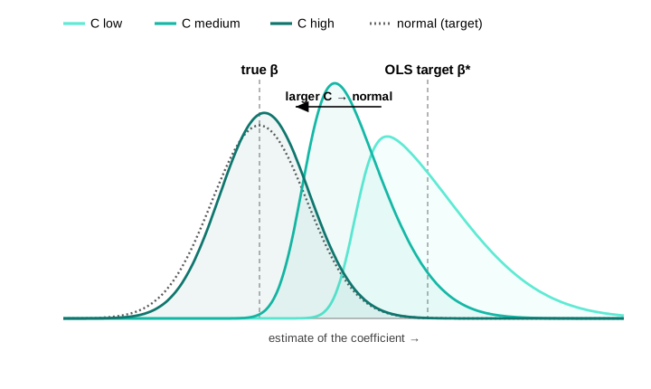
- Each \(\mathbf{C}\) is one curve. Small \(\mathbf{C}\) (weak first stage): skewed, heavy-tailed, shoved toward the OLS bias at \(\bbeta^{*}\). As \(\mathbf{C}\) grows the density marches back onto the normal at \(\bbeta\).
- The textbook normal is the \(\mathbf{C}\to\infty\) edge — and its sample read-out is the first-stage \(F\): low \(F\) puts you on a left-shifted curve, high \(F\) on the normal.
Bias toward OLS, and the concentration parameter
A weak first stage drags 2SLS back toward the OLS bias it was meant to remove. How strong the first stage is gets summarised by one number — the concentration parameter \(\mu^2\), a signal-to-noise measure of the first stage. Big \(\mu^2\) = strong instrument; in practice you read it off the first-stage \(F\).
- Weak \(\Rightarrow\) 2SLS inherits the OLS bias. The smaller \(\mu^2\), the more of the OLS bias survives — as \(\mu^2\to0\), 2SLS is OLS.
- Many weak instruments make it worse. Each extra weak instrument adds noise, not signal — strength beats count: a few strong instruments beat many weak ones.
- In practice you never compute \(\mu^2\); you judge first-stage strength by the \(F\)-statistic (next slide).
Diagnosis and honest inference
The first-stage F — and why \(F>10\) is not enough
The first-stage \(F\) (joint significance of the excluded instruments) estimates \(\mu^2\) via \(\E[F]\approx1+\mu^2/\ell\), so \(\mu^2\approx\ell(F-1)\). Why the famous threshold 10? The 2SLS relative bias is \(\approx\ell/(\mu^2+\ell)=1/\E[F]\approx 1/F\) — so \(F=10\) caps it at about 10%:
| first-stage \(F\) | \(\mu^2\ (\ell=1)\) | 2SLS bias \(\approx 1/F\) |
|---|---|---|
| 2 | 1 | 50% |
| 5 | 4 | 20% |
| 10 | 9 | 10% |
| 20 | 19 | 5% |
- But \(F>10\) controls the bias, not the \(t\)-test. For an honest 5% \(t\)-test you need far more — effective \(F\approx104.7\), two orders above the folklore (Lee et al. 2022).
- Report \(F\), but do not treat \(F>10\) as a clean bill of health — when in doubt, use weak-robust inference (next slide).
Weak-robust inference: Anderson–Rubin
The fix is inference that is valid whatever the instrument strength. The workhorse is the Anderson–Rubin (AR) test of a candidate value \(\bbeta_0\): if \(\bbeta_0\) is the truth, the imposed residual \(y-\mathbf{x}'\bbeta_0\) is just the exogenous error, so the instruments should have no power to predict it — regress it on them and test exactly that.
- AR statistic: \(F\)-test of \(\boldsymbol{\gamma}=\mathbf{0}\) in \(\,y_i-\mathbf{x}_i'\bbeta_0=\mathbf{z}_i'\boldsymbol{\gamma}+u_i\) — exact under normality, asymptotically \(\chi^2_\ell/\ell\), and does not depend on \(\boldsymbol{\Pi}\).
- Weak-robust confidence set = all \(\bbeta_0\) the AR test does not reject (invert the test). It can be bounded, empty, or infinite — honestly reflecting what the data identify.
- Over-identified refinements: AR wastes power when \(\ell>k\); the conditional likelihood ratio (CLR) test is the near-optimal choice (Moreira 2003). Just-identified: AR is already efficient.
The cautionary tale
Angrist–Krueger (1991) instrumented schooling with quarter of birth interacted with year and state — hundreds of individually weak instruments. Bound, Jaeger & Baker showed the 2SLS estimates were biased toward OLS, and — the famous demonstration — that replacing quarter of birth with randomly generated instruments produced similar, deceptively “precise” 2SLS estimates. A large sample (\(n\approx 300{,}000\)) gave no protection. This paper launched the weak-instrument literature (Bound et al. 1995).
The weak-instrument diagnosis is the mirror image of Lecture 9’s rank condition: there, \(\rank(\E[\mathbf{z}\mathbf{x}'])=k\) was identification in the population; here, a first stage that is full-rank but tiny is the practical failure. Strong identification is a quantitative version of the rank condition.
Part III · Specification tests
Do we need IV, and are the instruments consistent?
Testing endogeneity: Hausman–Wu
If \(\mathbf{x}\) were exogenous, OLS and IV would both be consistent and OLS would be efficient (Part I). A large gap between them is therefore evidence of endogeneity.
- Hausman statistic: \((\bb_{\text{IV}}-\bb_{\text{OLS}})'\big[\widehat{\Var}(\bb_{\text{IV}})-\widehat{\Var}(\bb_{\text{OLS}})\big]^{-1}(\bb_{\text{IV}}-\bb_{\text{OLS}})\dto\chi^2_{k_2}\) under \(H_0\) (exogeneity) (Hausman 1978).
- Regression (control-function) form — easier and robust: add the first-stage residual \(\hat{\mathbf{v}}\) to the structural OLS, \(y=\mathbf{x}'\bbeta+\hat{\mathbf{v}}'\boldsymbol{\rho}+\text{error}\); a \(t\)/\(F\)-test of \(\boldsymbol{\rho}=\mathbf{0}\) is the endogeneity test.
- Reject ⇒ keep IV; fail to reject ⇒ OLS is consistent and more precise — prefer it. (But a weak first stage saps the test’s power.)
Testing overidentification: Sargan / Hansen
When \(\ell>k\) there are more moment conditions than parameters, so the instruments can be checked against each other: if all are valid, the 2SLS residuals should be (nearly) orthogonal to every instrument.
- Sargan statistic: \(n\cdot R^2\) from regressing the 2SLS residuals \(\hat\varepsilon\) on \(\mathbf{z}\), distributed \(\chi^2_{\ell-k}\) under \(H_0\) (all instruments valid) (Sargan 1958); the heteroskedastic-robust version is the GMM \(J\)-test of Lecture 11.
- Reject ⇒ the overidentifying restrictions are mutually inconsistent — some instrument fails exclusion (or the model is misspecified).
- Three caveats: it tests the instruments jointly (not which one fails); it has low power; and it can say nothing about the \(k\) instruments needed for identification — a just-identified model is untestable this way.
Summary
What to take away
- IV buys consistency under endogeneity at a price in variance: when \(\mathbf{x}\) is exogenous, OLS is consistent and more efficient — so do not use IV reflexively.
- 2SLS is asymptotically \(\Normal(\mathbf{0},\bV)\) with a sandwich variance; use a proper 2SLS command for robust/clustered standard errors.
- Weak instruments — a first stage small relative to noise — bias 2SLS toward OLS, break normality, and invalidate the usual \(t\) and CI. More (weak) instruments make it worse.
- Report the first stage \(F\), but know \(F>10\) controls bias, not the \(t\)-test; when in doubt use weak-robust inference (Anderson–Rubin / CLR), which is valid at any instrument strength.
- Specification tests: Hausman–Wu asks do we need IV?; Sargan/Hansen asks are the surplus instruments mutually consistent? — but exclusion of the core instruments stays an untestable design argument.