Endogeneity and Identification by Instrumental Variables
Lecture 9
PIMES/UFPE
Where we are
Where this lecture sits
For eight lectures, one assumption carried every consistency result: exogeneity, \(\E[\mathbf{x}_i\varepsilon_i]=\mathbf{0}\). This lecture asks what happens when it fails — when a regressor is correlated with the error. Least squares then breaks in the limit, not merely in small samples. Naming that failure is endogeneity; repairing it needs information from outside the regression — an instrument. At heart it is a question of identification: with exogeneity gone, is the parameter still recoverable?
What least squares actually estimates
A refresher from Lecture 2 — with no assumptions beyond finite second moments.
- A population object: among all linear predictors \(\mathbf{x}'b\), the best in mean square is \(\bbeta^{*}=(\E[\mathbf{x}\mathbf{x}'])^{-1}\E[\mathbf{x}y]\) — a fixed feature of the distribution \(F\), defined with no data.
- Its defining property: the projection error \(u=y-\mathbf{x}'\bbeta^{*}\) is orthogonal to \(\mathbf{x}\) by construction, \(\E[\mathbf{x}u]=\mathbf{0}\) (not an assumption).
- OLS is its sample analogue: replace \(\E[\cdot]\) by sample averages, giving \(\bb=(\bX'\bX)^{-1}\bX'\bY\); by the LLN \(\bb\pto\bbeta^{*}\), with no exogeneity and no causal story.
- So consistency is never in doubt — the real question is consistent for what?
Part I · Structural vs. projection
Endogeneity
When the projection is not the parameter
Definition 1 (Endogeneity) Posit a structural equation \(y_i=\mathbf{x}_i'\bbeta+\varepsilon_i\) in which \(\bbeta\) is defined by economics — the causal effect — not by fit. A regressor is endogenous for \(\bbeta\) when it is correlated with the structural error, equivalently when the structural parameter and the projection disagree: \[\E[\mathbf{x}_i\varepsilon_i]\neq\mathbf{0}\iff\bbeta^{*}\neq\bbeta.\] It is a property relative to a structural equation — the same variable can be exogenous in one model and endogenous in another.
- Two coefficients now live in one regression: the projection \(\bbeta^{*}\) (what OLS estimates) and the structural \(\bbeta\) (what we want).
- The key contrast: the projection error \(u=y-\mathbf{x}'\bbeta^{*}\) is orthogonal to \(\mathbf{x}\) always; the structural error \(\varepsilon=y-\mathbf{x}'\bbeta\) is orthogonal to \(\mathbf{x}\) only under exogeneity. Endogeneity is when \(\varepsilon\) still carries part of \(\mathbf{x}\).
- Exogenous \(\Rightarrow\bbeta^{*}=\bbeta\) (the world of Lectures 4–8); endogenous \(\Rightarrow\bbeta^{*}\neq\bbeta\).
- Which one you intend is an economic question — the data alone cannot tell \(\bbeta\) from \(\bbeta^{*}\).
A concrete case: the return to schooling
Regress log weekly earnings on years of education (plus experience and controls). OLS gives a return of about 7% per year — clean and precise. Is it the causal return?
- Education is a choice: abler people tend to get more schooling and earn more anyway.
- Ability is unobserved, so it sits in the error \(\varepsilon\) — and it is correlated with schooling: \(\E[\mathbf{x}_i\varepsilon_i]\neq\mathbf{0}\).
- So the \(7\%\) is the projection \(\bbeta^{*}\), inflated by ability — not the structural return \(\bbeta\). The fix comes in Part II.
Why OLS is inconsistent for \(\bbeta\)
With \(\bb=(\bX'\bX)^{-1}\bX'\bY\) and the structural \(\bY=\bX\bbeta+\beps\),
\[\bb =\bbeta+\Big(\tfrac1n\textstyle\sum_i\mathbf{x}_i\mathbf{x}_i'\Big)^{-1}\Big(\tfrac1n\textstyle\sum_i\mathbf{x}_i\varepsilon_i\Big) \;\pto\;\underbrace{\bbeta+\big(\E[\mathbf{x}_i\mathbf{x}_i']\big)^{-1}\E[\mathbf{x}_i\varepsilon_i]}_{=\;\bbeta^{*}}.\]
- OLS lands exactly on the projection \(\bbeta^{*}\) — it does its job perfectly.
- Under exogeneity the last term is \(\mathbf{0}\) and \(\bbeta^{*}=\bbeta\); under endogeneity it does not vanish.
- So \(\bb\pto\bbeta^{*}\neq\bbeta\): more data only sharpens the estimate of the wrong object — inconsistency, not bias.
The DGP, from here on
The population is \(\{(y_i,\mathbf{x}_i,\mathbf{z}_i)\}\), i.i.d. from \(F\). The structural equation is \(y_i=\mathbf{x}_i'\bbeta+\varepsilon_i\), but now \(\E[\mathbf{x}_i\varepsilon_i]\neq\mathbf{0}\) for at least one regressor. Alongside \(\mathbf{x}\) there is a further variable \(\mathbf{z}\) — the instrument, developed in Part II — whose role is to supply the identifying information the structural equation lacks on its own.
- Population: i.i.d. draws \((y_i,\mathbf{x}_i,\mathbf{z}_i)\) from an unknown \(F\) — nothing observed but these.
- Structural equation \(y_i=\mathbf{x}_i'\bbeta+\varepsilon_i\), with \(\bbeta\) the causal target — but at least one regressor is endogenous, \(\E[\mathbf{x}_i\varepsilon_i]\neq\mathbf{0}\).
- The instrument \(\mathbf{z}_i\): an extra variable carrying identifying information from outside the equation — the conditions that qualify it come in Part II.
Four sources of endogeneity
Four roads to \(\bbeta^{*}\neq\bbeta\)
- Omitted variables — a determinant of \(y\), correlated with \(\mathbf{x}\), is left in the error (schooling and ability).
- Measurement error — \(\mathbf{x}\) is observed with noise.
- Sample selection — the sample is chosen in a way related to \(\varepsilon\).
- Simultaneity — \(y\) and \(\mathbf{x}\) are determined jointly (supply and demand).
Omitted variables
The long model is \(y_i=\mathbf{x}_i'\bbeta+w_i\gamma+u_i\), with \(u\) orthogonal to both \(\mathbf{x}\) and \(w\). Omit \(w\) and it falls into the error, \(\varepsilon_i=w_i\gamma+u_i\), giving \(\E[\mathbf{x}_i\varepsilon_i]=\gamma\,\E[\mathbf{x}_i w_i]\).
- Our running case: schooling and ability — abler people get more schooling and earn more.
- The omitted-variable bias is \(\bbeta^{*}-\bbeta=\gamma\,(\E[\mathbf{x}\mathbf{x}'])^{-1}\E[\mathbf{x} w]\) — nonzero exactly when \(w\) matters (\(\gamma\neq0\)) and covaries with \(\mathbf{x}\).
- Sign (scalar \(x\)): \(\bbeta^{*}=\bbeta+\gamma\,\Cov(x,w)/\Var(x)\) — ability raises wages (\(\gamma>0\)) and covaries positively with schooling, so OLS overstates the return.
The long-vs-short coefficient gap \(\gamma\,(\E[\mathbf{x}\mathbf{x}'])^{-1}\E[\mathbf{x} w]\) is the omitted-variable bias of Lecture 3. Omitted-variable bias is endogeneity, seen from the regression table.
Measurement error: attenuation
We regress on a noisy measurement \(\tilde x_i=x_i^{*}+u_i\) of the true regressor \(x_i^{*}\), with \(u_i\) independent of \(x_i^{*}\) and \(\varepsilon_i\). The structural model is \(y_i=x_i^{*}\beta+\varepsilon_i\), so in terms of \(\tilde x_i\) the error becomes \(\varepsilon_i-\beta u_i\) and
\[\plim b=\beta^{*} =\beta\,\frac{\Var(x_i^{*})}{\Var(x_i^{*})+\Var(u_i)} =\frac{\beta}{1+\Var(u_i)/\Var(x_i^{*})}\;<\;\beta.\]
- Classical measurement error attenuates: the projection \(\beta^{*}\) is pulled toward zero, by the noise-to-signal ratio.
- The noisier the regressor, the stronger the pull — and it does not wash out as \(n\to\infty\).
This is the inconsistent estimator from the Monte Carlo taxonomy (Demo 2): the sampling distribution tightened on the wrong value, \(0.5\) rather than \(\beta=1\). There we saw it; here we derive it.
Sample selection
Even when \(\mathbf{x}\) is exogenous in the full population, keeping only the units that made it into the sample can make the in-sample error correlated with \(\mathbf{x}\).
- Conditioning on being selected leaves \(\E[\mathbf{x}\varepsilon\mid\text{selected}]\neq\mathbf{0}\) — whatever decides who enters the sample sits in the error and moves with \(\mathbf{x}\).
- Many guises: self-selection (wages only for workers), attrition (tracked units that drop out), survivorship (only survivors in the data), truncation/censoring (approved loans, top-coded income — recorded only up to a cap).
- Same mechanism as the others — it is omitted-variable bias: the missing “selection correction” is the omitted regressor (the formal, Heckman version is in the notes).
Simultaneity
Price and quantity are set together — demand and supply hold at once: \[q_i=\alpha p_i+\varepsilon_i^{d}\ (\text{demand}),\qquad q_i=\delta p_i+\varepsilon_i^{s}\ (\text{supply}).\]
- The equilibrium price solves both equations, so it carries both shocks: \(p_i=(\varepsilon_i^{s}-\varepsilon_i^{d})/(\alpha-\delta)\) — hence \(\E[p_i\varepsilon_i^{d}]\neq0\), \(p\) endogenous in either equation.
- Regressing \(q\) on \(p\) recovers neither slope: \(\plim b=(\alpha\sigma_s^2+\delta\sigma_d^2)/(\sigma_s^2+\sigma_d^2)\) — a variance-weighted blend of the two (the identification problem, Working 1927).
- The fix, in one picture: a variable \(z\) that shifts supply only (an input cost, absent from demand) moves supply along the fixed demand curve — the equilibria then trace out demand, and \(z\) identifies \(\alpha\). This is the instrument, and IV was born here (Wright, 1928) — the bridge to Part II.
Part II · Identification by an instrument
What identification means
When is a parameter identified?
Definition 2 (Identification) A parameter is identified if it is a unique function of the distribution of the observables. The projection \(\bbeta^{*}\) is always identified — it is an explicit function of population moments. The structural \(\bbeta\) is identified only if the data pin it down uniquely; under endogeneity the structural equation alone does not, so we must add information.
To pin down \(\bbeta\) (\(k\) unknowns) you need \(k\) valid moment conditions \(\E[\mathbf{w}(y-\mathbf{x}'\bbeta)]=\mathbf{0}\) — a solvable linear system: \[\E[\mathbf{w}\,y]=\E[\mathbf{w}\,\mathbf{x}']\,\bbeta,\qquad\text{unique }\bbeta\iff \rank\big(\E[\mathbf{w}\mathbf{x}']\big)=k.\]
- With only \((y,\mathbf{x})\): the lone candidate \(\mathbf{w}=\mathbf{x}\) is invalid (\(\E[\mathbf{x}\varepsilon]\neq\mathbf{0}\)) — it returns \(\bbeta^{*}\), not \(\bbeta\). No valid full-rank moment \(\Rightarrow\bbeta\) not identified.
- A relevant, exogenous \(\mathbf{z}\) (\(\E[\mathbf{z}\varepsilon]=\mathbf{0}\)) restores it: \(\E[\mathbf{z}y]=\E[\mathbf{z}\mathbf{x}']\bbeta\), identified iff \(\rank(\E[\mathbf{z}\mathbf{x}'])=k\) — the relevance/rank condition.
- Identification is prior to estimation: rank deficient \(\Rightarrow\) no estimator recovers \(\bbeta\) at any \(n\) (preview of weak instruments, Lecture 10).
What an instrument is
Two conditions
Definition 3 (Instrumental variable) A variable \(\mathbf{z}_i\) is a valid instrument for an endogenous \(\mathbf{x}_i\) if it satisfies
- Relevance: \(\Cov(\mathbf{z}_i,\mathbf{x}_i)\neq 0\) — it moves the endogenous regressor; and
- Exogeneity (exclusion): \(\E[\mathbf{z}_i\varepsilon_i]=\mathbf{0}\) — it is unrelated to the error, affecting \(y\) only through \(\mathbf{x}\).
- Relevance is about the first stage — testable, and the subject of “weak instruments” next lecture.
- Exclusion is about the DGP — an identification assumption the data cannot verify.
- A good instrument is a source of variation in \(\mathbf{x}\) that is as good as randomly assigned.
Relevance and exclusion, in words
Think of the instrument as a lever on \(\mathbf{x}\).
- Relevance — the lever is connected: pulling \(\mathbf{z}\) actually moves \(\mathbf{x}\), \(\Cov(\mathbf{z},\mathbf{x})\neq0\). Checked against the sample (the first stage).
- Exclusion — the lever reaches \(y\) through no other wire than \(\mathbf{x}\): hold \(\mathbf{x}\) fixed and \(\mathbf{z}\) says nothing more about \(y\). An economic argument, not a test.
- The two do opposite jobs, checked by opposite means — relevance against data, exclusion against theory.
- It is why IV papers live or die on the story for exclusion, not a statistic.
The IV causal diagram
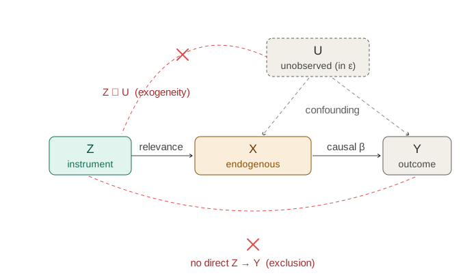
- Present: \(\mathbf{z}\to\mathbf{x}\) (relevance), \(\mathbf{x}\to y\) (the causal \(\bbeta\)), and \(U\to\mathbf{x}\), \(U\to y\) (confounding — why \(\mathbf{x}\) is endogenous).
- Forbidden (red): a direct \(\mathbf{z}\to y\) (exclusion) and any \(\mathbf{z}\!-\!U\) link (exogeneity).
- With both absent, the variation in \(\mathbf{x}\) driven by \(\mathbf{z}\) is as good as random — and that slice identifies \(\bbeta\).
Exogeneity as a moment condition
The condition that defines the estimator
Write exclusion as an expectation involving the parameter: \[\E\big[\mathbf{z}_i(y_i-\mathbf{x}_i'\bbeta)\big]=\E[\mathbf{z}_i\varepsilon_i]=\mathbf{0}.\] This single vector equation is the estimator — replace the expectation by its sample analogue and solve. For OLS the instrument is \(\mathbf{x}\) itself (\(\E[\mathbf{x}_i\varepsilon_i]=\mathbf{0}\)); when \(\mathbf{x}\) is endogenous we swap in \(\mathbf{z}\). This is the moment condition that returns, generalised to \(\E[g(W_i,\theta)]=\mathbf{0}\), as the foundation of GMM in Lecture 11.
- Same equation, different instrument: OLS imposes \(\E[\mathbf{x}_i\varepsilon_i]=\mathbf{0}\) (\(\mathbf{x}\) instruments itself); IV imposes \(\E[\mathbf{z}_i\varepsilon_i]=\mathbf{0}\) (\(\mathbf{z}\) in place of \(\mathbf{x}\)).
- One moment condition per instrument: \(\ell\) equations (\(\ell=\dim\mathbf{z}\)) for the \(k\) unknowns in \(\bbeta\) (\(k=\dim\mathbf{x}\)).
- The count decides everything: \(\ell=k\) gives the IV estimator; \(\ell>k\) needs 2SLS. But which columns are \(\mathbf{x}\), what goes into \(\mathbf{z}\), and when does the count hold? — right below.
Which columns are endogenous — and what goes into \(\bZ\)
Split the \(k\) regressors by their relation to the error, then build the instrument vector to match: \[\mathbf{x}_i=\begin{pmatrix}\mathbf{x}_{1i}\\[2pt]\mathbf{x}_{2i}\end{pmatrix},\qquad \underbrace{\E[\mathbf{x}_{1i}\varepsilon_i]=\mathbf{0}}_{k_1\text{ exogenous}},\quad \underbrace{\E[\mathbf{x}_{2i}\varepsilon_i]\neq\mathbf{0}}_{k_2\text{ endogenous}},\qquad k=k_1+k_2,\] \[\mathbf{z}_i=\begin{pmatrix}\mathbf{x}_{1i}\\[2pt]\mathbf{z}_{2i}\end{pmatrix},\qquad \underbrace{\mathbf{x}_{1i}}_{\text{included }(\ell_1=k_1)},\quad \underbrace{\mathbf{z}_{2i}}_{\text{excluded }(\ell_2)},\qquad \ell=\ell_1+\ell_2,\ \ \ell_1=k_1.\]
- Exogenous regressors instrument themselves. The \(k_1\) clean columns \(\mathbf{x}_1\) enter \(\bZ\) unchanged — they already satisfy \(\E[\mathbf{x}_1\varepsilon]=0\), so there is nothing to replace. These are the included instruments — \(\ell_1=k_1\) of them.
- Only the \(k_2\) endogenous columns need help. For them we bring in \(\ell_2\) excluded instruments \(\mathbf{z}_2\) — variables deliberately kept out of the structural equation (that absence is the exclusion restriction) that still move \(\mathbf{x}_2\).
- Counting — the order condition. \(\ell\) moment equations for \(k\) parameters ⇒ need \(\ell\ge k\); since the \(k_1\) exogenous slots line up automatically, this is just \(\ell_2\ge k_2\) — at least as many excluded instruments as endogenous regressors.
- \(\ell_2=k_2\ (\ell=k)\): exactly identified → IV, \(\bZ'\bX\) square.
- \(\ell_2>k_2\ (\ell>k)\): over-identified → 2SLS (next).
- \(\ell_2<k_2\): under-identified → no consistent estimator.
Reduced form and first stage
The first stage
The first stage regresses the endogenous regressor on the instruments, \[\mathbf{x}_i=\boldsymbol{\Pi}'\mathbf{z}_i+\mathbf{v}_i,\qquad \boldsymbol{\Pi}=(\E[\mathbf{z}\mathbf{z}'])^{-1}\E[\mathbf{z}\mathbf{x}'].\] Substituting into the structural equation gives the reduced form of \(y\), \[y_i=\mathbf{z}_i'(\boldsymbol{\Pi}\bbeta)+(\mathbf{v}_i'\bbeta+\varepsilon_i),\] a regression of \(y\) on the exogenous \(\mathbf{z}\) — consistently estimable by OLS.
- Why OLS on \(\mathbf{z}\) is clean: the composite error \(\mathbf{v}'\bbeta+\varepsilon\) is orthogonal to \(\mathbf{z}\) — \(\mathbf{z}\perp\mathbf{v}\) (the first stage is a projection: \(\mathbf{v}=\mathbf{x}-\boldsymbol{\Pi}'\mathbf{z}\perp\mathbf{z}\) by construction) and \(\mathbf{z}\perp\varepsilon\) (exogeneity). But \(\mathbf{x}\) is not clean — \(\Cov(\mathbf{v},\varepsilon)\neq0\) is the endogeneity.
- Relevance = the rank condition: \(\boldsymbol{\Pi}\) has full column rank \(k\iff\rank(\E[\mathbf{z}\mathbf{x}'])=k\) (as \(\E[\mathbf{z}\mathbf{z}']\) is invertible, \(\rank\boldsymbol{\Pi}=\rank\E[\mathbf{z}\mathbf{x}']\)) — exactly the identification condition from before.
- First stage (\(\boldsymbol{\Pi}\)) = how much \(\mathbf{z}\) moves \(\mathbf{x}\); reduced form (\(\boldsymbol{\lambda}=\boldsymbol{\Pi}\bbeta\)) = the total effect of \(\mathbf{z}\) on \(y\) — which, by exclusion, runs entirely through \(\mathbf{x}\) (the only path \(\mathbf{z}\to\mathbf{x}\to y\)).
- So IV = reduced form ÷ first stage: \(\bbeta=\boldsymbol{\lambda}/\boldsymbol{\Pi}\) (scalar) — the \(\mathbf{z}\to y\) effect over the \(\mathbf{z}\to\mathbf{x}\) effect.
Part III · The IV and 2SLS estimators
Exactly identified
The IV estimator
Definition 4 (IV estimator (exactly identified)) When \(\ell=k\) (exactly identified: \(\ell_2=k_2\) excluded instruments for the \(k_2\) endogenous regressors, with \(\mathbf{x}_1\) instrumenting itself), the sample moment condition \(\tfrac1n\sum_i\mathbf{z}_i(y_i-\mathbf{x}_i'\mathbf{b})=\mathbf{0}\) solves uniquely: \[\bb_{\text{IV}}=(\bZ'\bX)^{-1}\bZ'\bY,\qquad\text{scalar: } b_{\text{IV}}=\frac{\Cov(z,y)}{\Cov(z,x)}=\frac{\lambda}{\Pi}.\] The scalar form is literally reduced form \(\div\) first stage — \(\lambda=\) effect of \(z\) on \(y\), \(\Pi=\) effect of \(z\) on \(x\).
- Read it as \(\lambda/\Pi\): the \(z\to y\) effect over the \(z\to x\) effect. Since \(z\) reaches \(y\) only through \(x\), dividing isolates the \(x\to y\) effect \(\bbeta\).
- Consistent for the structural \(\bbeta\): exclusion (\(\E[\mathbf{z}\varepsilon]=0\)) kills the error term, relevance (\(\E[\mathbf{z}\mathbf{x}']\) invertible) makes the formula well-defined.
- The limit it rests on: \(\tfrac1n\bZ'\bX\pto\mathbf{Q}_{zx}\equiv\E[\mathbf{z}\mathbf{x}']\), a finite, invertible matrix (regularity + relevance) — so \((\tfrac1n\bZ'\bX)^{-1}\pto\mathbf{Q}_{zx}^{-1}\) and, with \(\tfrac1n\bZ'\beps\pto\mathbf{0}\), Slutsky gives \(\bb_{\text{IV}}\pto\bbeta\).
- A weak first stage (\(\Pi\approx0\)) is a near-zero denominator — the estimator turns fragile (Lecture 10).
- Set \(\mathbf{z}=\mathbf{x}\) and IV collapses to OLS: OLS is just IV with \(x\) instrumenting itself.
Overidentified
Two-stage least squares
With \(\ell>k\) instruments (\(\ell_2>k_2\) excluded ones), each gives a valid IV — but one at a time wastes the others. Any linear combination of the \(\mathbf{z}\)’s is still a valid instrument; the best (most correlated with \(\mathbf{x}\)) is the first-stage OLS fit. Hence literally two OLS stages: \[\textbf{Stage 1: } \hat{\bX}=\bP_{\bZ}\bX,\quad \bP_{\bZ}=\bZ(\bZ'\bZ)^{-1}\bZ';\qquad \textbf{Stage 2: } \bb_{\text{2SLS}}=(\hat{\bX}'\hat{\bX})^{-1}\hat{\bX}'\bY.\] Since \(\bP_{\bZ}\) is symmetric and idempotent (\(\hat{\bX}'\hat{\bX}=\bX'\bP_{\bZ}\bX\), \(\hat{\bX}'\bY=\bX'\bP_{\bZ}\bY\)): \[\bb_{\text{2SLS}}=(\bX'\bP_{\bZ}\bX)^{-1}\bX'\bP_{\bZ}\bY.\]
- Why not just pick one? Each valid \(\mathbf{z}\) gives a consistent IV, but using one throws away the information in the excluded instruments.
- Stage 1 builds the best combined instrument — regress \(\mathbf{x}\) on all \(\mathbf{z}\) → fitted \(\hat{\mathbf{X}}=\bP_{\bZ}\bX\); Stage 2 regresses \(y\) on \(\hat{\mathbf{X}}\). Idempotency of \(\bP_{\bZ}\) folds the two into one formula.
- Exactly identified (\(\ell=k\)) → 2SLS equals IV (proof below); the projection is the general, over-identified (\(\ell>k\)) case.
What the two stages actually do
- Stage 1 isolates the clean part of \(\mathbf{x}\): \(\hat{\mathbf{X}}=\bP_{\bZ}\bX\) keeps only the variation driven by \(\mathbf{z}\) — orthogonal to \(\varepsilon\) by exclusion.
- Stage 2 regresses \(y\) on that trustworthy variation, discarding the endogenous part that is tangled with the error.
- 2SLS trades information for honesty: it uses only the slice of \(\mathbf{x}\)’s variation it can trust.
Estimating the two OLS regressions separately gives the right point estimate but the wrong standard errors — the second stage treats \(\hat{\bX}\) as data and ignores that it was estimated. Always use a 2SLS command (ivreg, feols(... | ...), ivregress), which corrects the variance.
Part IV · Endogenous dummies and treatment effects
A binary endogenous regressor
Let \(D_i\in\{0,1\}\) be an endogenous treatment (people select into it) and \(z_i\in\{0,1\}\) a binary instrument. The IV estimator becomes the Wald estimator, \[b_{\text{IV}}=\frac{\bar y_{\,z=1}-\bar y_{\,z=0}}{\bar D_{\,z=1}-\bar D_{\,z=0}} =\frac{\text{reduced-form effect of }z\text{ on }y}{\text{first-stage effect of }z\text{ on }D}.\]
- The same \(\lambda/\Pi\) estimator, \(b_{\text{IV}}=\Cov(z,y)/\Cov(z,x)\): with \(z\in\{0,1\}\) each covariance is a difference in means — numerator = how \(y\) differs across groups, denominator = how treatment differs.
- Dividing rescales the reduced-form effect of \(z\) into a per-unit-of-treatment effect.
- With heterogeneous effects it is a local effect — the average effect on the compliers the instrument moves (the LATE, next).
Oversubscribed KIPP charter schools admit by lottery: winning the lottery \(z\in\{0,1\}\) is randomly assigned, a textbook-clean instrument for actually attending \(D\in\{0,1\}\) (not every winner enrols, and losers rarely attend). 2SLS of test scores on attendance, instrumented by the lottery offer, estimates KIPP’s effect — a LATE for the students whose enrolment the lottery moves (Angrist et al. 2012). (Angrist–Krueger’s quarter-of-birth returns in Lecture 10 as the weak-instrument cautionary tale.)
Heterogeneous effects: the LATE
Who does the instrument move?
Label each unit by how its treatment would respond to the binary instrument — its potential treatments \((D_i(0),D_i(1))\). Read through the Vietnam draft (Angrist 1990): \(z=\) draft-eligible (random lottery number), \(D=\) served, \(y=\) earnings.
| \(D_i(0)\,\backslash\,D_i(1)\) | \(D_i(1)=0\) | \(D_i(1)=1\) |
|---|---|---|
| \(D_i(0)=0\) | never-taker | complier |
| \(D_i(0)=1\) | defier | always-taker |
- Compliers (\(0\to1\)): serve because drafted — the only group the instrument actually moves.
- Always-takers (\(1,1\)): volunteers, serve either way. Never-takers (\(0,0\)): unfit/deferred, never serve. The instrument changes neither.
- Defiers (\(1\to0\)): would serve only if not drafted — implausible; monotonicity assumes they do not exist.
The Wald ratio is a LATE
Under random \(z\), exclusion, relevance, and monotonicity (no defiers), the Wald ratio identifies the average treatment effect on compliers: \[\frac{\E[y\mid z=1]-\E[y\mid z=0]}{\E[D\mid z=1]-\E[D\mid z=0]}=\E[\,y_1-y_0\mid\text{complier}\,]\equiv\textbf{LATE}.\]
- Denominator = share of compliers: \(\E[D\mid z{=}1]-\E[D\mid z{=}0]\) is exactly the fraction whose treatment the instrument flips.
- Numerator = compliers only: always- and never-takers keep the same \(D\) under \(z=0,1\), so by random \(z\) their \(y\) cancels; only compliers switch.
- So IV \(\neq\) ATE: it is local — silent on always- and never-takers. A different instrument moves a different complier group → a different LATE.
Summary
What to take away
- OLS always estimates the projection \(\bbeta^{*}\); endogeneity (\(\E[\mathbf{x}\varepsilon]\neq\mathbf{0}\), i.e. \(\bbeta^{*}\neq\bbeta\)) makes it inconsistent for the structural \(\bbeta\) — wrong target, not small-sample bias.
- Four sources, one symptom: omitted variables, measurement error, selection, simultaneity.
- Recovering \(\bbeta\) is identification, not estimation: an instrument with relevance (\(\Cov(\mathbf{z},\mathbf{x})\neq0\)) and exclusion (\(\E[\mathbf{z}\varepsilon]=\mathbf{0}\)) makes \(\bbeta\) a unique function of observable moments.
- Exactly identified (\(\ell=k\), i.e. \(\ell_2=k_2\)) → \(\bb_{\text{IV}}=(\bZ'\bX)^{-1}\bZ'\bY\); overidentified (\(\ell>k\)) → 2SLS projects \(\bX\) onto \(\bZ\).
- IV buys consistency; the price — efficiency, and total reliance on an untestable exclusion — is next lecture.
Hansen, Econometrics, ch. 12; Greene, ch. 8.